Some novel observations on organ pipe sounds and their frequency spectra
Colin Pykett
Posted: 26
November 2015
Revised: 17
June 2021
Copyright © C E Pykett
Abstract.
This
article shows that the four classes of organ pipe tone - flutes, diapasons
(or principals), strings and reeds - have frequency spectra characterised by significant amplitude scatter which
often obscures their
systematic structure. It is therefore remarkable that
our ears have little difficulty in deciding that the sounds from a given rank of
pipes belong to the same stop on an organ. However groupings of
harmonics have been identified in the spectra analysed
over some forty years of research, and each can be associated with a
linear trendline fitted to the harmonics of its group. Using additive synthesis it has been found that
the subjective tone quality of a pipe is little changed when it is
reconstructed from its trendline values rather than from its actual harmonic
amplitudes.
In any case, such differences as do exist between the actual sound of a pipe and
its reconstruction are often eclipsed by those occurring naturally
between adjacent pipes owing to the gross variations in their spectra. In most
cases only two trendlines are required in each spectrum.
This
finding might be significant in aural perception because it is a means of reducing the confusing welter of data in
real spectra to a much simpler generic form which nonetheless retains the essentials of the sound of
an organ pipe which satisfies the ear. Because the ear and brain process
both amplitude and frequency logarithmically, the trendlines themselves on a similar log-log spectrum plot take the simplest possible form,
namely straight lines rather than curves. This being so, each trendline is
defined using
only two parameters - its slope and its intercept on the amplitude axis.
Thus a spectrum with an arbitrary number of harmonics can be reduced to just
four numbers which nevertheless seem to encode its essential subjective features. This represents a considerable dimensionality reduction
in a spectrum with many harmonics which has implications for acoustic pattern
recognition, whether implemented by brains or machines.
It
is well-established that brains extract linear features when
processing visual sensory inputs, and it is therefore possible that similar neural
mechanisms might operate when processing the auditory sensory data arriving from
the inner ear. An amplitude-frequency spectrum is merely a 'picture' which
must be projected within the auditory cortex in some way, and it is conceivable
that linear features within it - such as the trendlines discussed here -
are extracted as part of the acoustic pattern recognition processes in the
brain. There would seem to be implications for the mechanisms of musical perception in these
suggestions.
Contents
(click
on the headings below to access the desired section)
Introduction
The frequency spectra of Diapason pipes
Harmonic
Groups
Trendline
Analysis
The
frequency spectra of Flute pipes
The
frequency spectra of String pipes
The
frequency spectra of Reed pipes
Concluding
Remarks
Notes
and References
Introduction
It is well known that the tone quality or timbre of an organ pipe depends on the amplitudes of the harmonics which make up its frequency spectrum. However it is not unusual to find a spectrum which shows little systematic structure, with the amplitudes of adjacent harmonics jumping up and down relative to their neighbours so that the spectrum as a whole sometimes resembles little more than a scatter plot. This impression is amplified when one compares the spectra of two musically-adjacent organ pipes a semitone apart, which (should) sound subjectively similar apart from the difference in pitch, yet there is often little apparent similarity between the spectra evident to the eye. It is therefore remarkable that our ears and brain usually have little difficulty in deciding that the two pipes belong to the same organ stop. How is this aural feat performed when the harmonic structures of the two pipes can be so different?
Another oddity of organ tones is that some harmonics are far more important than others to the way we perceive the sounds. For example, using digital techniques it is
sometimes possible to delete certain harmonics completely, even the fundamental,
without making the slightest subjective difference to the sound of an organ pipe. On the other hand, the strengths of
other harmonics can be critical to the formation of an identifiable timbre and whether we consider it to be, say, a 'good' diapason tone or not.
It is also remarkable that pipe makers and voicers have learnt over many centuries how to adjust the amplitudes of these critical
harmonics using their ears alone.
This article addresses these fascinating phenomena. Among other things it trespasses into ways the ear and brain might extract meaningful features from the spectra, though it does not go very far, largely because it cannot as these processes are still imperfectly understood. An aspect pursued here is the spectral envelopes of the pipe sounds, illustrating how the harmonic amplitudes of organ pipes lie relative to one or more trendlines despite the apparent complexity of the spectra themselves. It is suggested that our auditory mechanism might extract simple line features such as these in a manner comparable to that which has been shown to exist in visual neural processing.
A large amount of information exists elsewhere on this website relating to the frequency spectra of organ pipes. Much of this is unique in two respects - such a comprehensive compendium of information can be found nowhere else, and it also embodies the results of a lot of original research on my part going back to the 1970s. It is impractical to attempt a summary here, so readers can browse as much or as little of it as they wish by referring to the other articles cited at reference
[1]. However it is perhaps useful to mention that there are four categories of organ stops - flutes, diapasons (or principals), strings and reeds. The first three use ranks of flue pipes of the type seen adorning the external casework of most instruments, whereas the last category employs pipes with vibrating reeds.
This article does not simply repeat the former material, as its aim was to look at frequency spectra in a novel manner which led to some interesting insights as to how we
might perceive organ sounds in the way we do.
The frequency spectra of Diapason
pipes
On a traditional church or concert organ anywhere in the world, the main foundation stop on which tonal mélanges are built is the Open Diapason or Principal at 8 foot pitch. This sound is unique to the organ because it exists nowhere else in musical experience, whereas stops comprising the other three categories (flutes, strings and reeds) often attempt to imitate other instruments, at least in name, though the results are not always convincing. So we shall commence by examining some Open Diapason spectra. It is tempting to fall into the trap of calling these 'typical' but, by virtue of what has just been said, there is in fact little typicality to be found and they are characterised more by their differences than their similarities. At the risk of becoming repetitious, the object is to try to understand why the ear discovers aural similarities so readily among these apparently disparate sound objects.
The frequency spectrum of an organ pipe is a graphical plot of the harmonics it emits when speaking, and the amplitude of each one.
Thus a spectrum is a sort of picture. Figure 1 shows the spectrum of the middle F sharp pipe of the Open Diapason on the Great Organ of the historic instrument at St Mary Ponsbourne in
Hertfordshire, England. I am grateful to the organist of the church, Paul
Minchinton, for making digital sound recordings available of each pipe on this instrument. The organ was built in 1858 by the well-known firm of J W Walker and its pipes still sound very acceptable today.
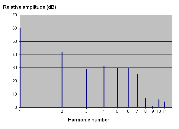
Figure 1. Spectrum of an Open Diapason pipe
(middle F#, Walker, 1858)
The frequency separation between adjacent pairs of harmonics is the same and equal to the fundamental frequency. However in this diagram, the harmonics are not uniformly spaced along the horizontal axis as might be expected because a logarithmic frequency scale has been used.
Further discussion of the logarithmic scales used for both axes on this graph is necessary, as it leads to some important consequences later on. The vertical axis illustrates the amplitude of each harmonic relative to that of the first and largest, which was set arbitrarily to 60 dB with the others being adjusted pro rata. Decibels are a logarithmic representation of ratios, and they have the useful feature that they compress a large range of numbers into a much smaller one. For example, the difference between 60 and 0 dB in this plot represents a ratio of 1000 to 1 in amplitude. Similarly, the dynamic range of the human ear is around 140 dB, corresponding to a ratio of 10,000,000 to 1 in sound pressure level
(SPL) between the quietest and loudest sounds we can safely perceive. Such numbers are too large to handle conveniently, either when plotting graphs or presumably within the neural circuits of the ear and brain. Their logarithms, numbers such as 60 or 140, are more manageable. Hence the use of logarithmic amplitude processing by the ear, and of decibels when plotting frequency spectra.
Our ears also process frequency logarithmically, frequency being the horizontal axis in Figure 1. However the harmonics in a spectrum are usually plotted linearly in frequency, so that the distance between adjacent pairs on the page is the same. Unfortunately this obscures some important insights which are only revealed when a logarithmic frequency scale is used, as here, and this is discussed later. A simple way to illustrate the logarithmic frequency processing used by the ear, which does not involve mathematics, merely requires that we consider an ordinary piano or organ keyboard. Its structure of repeating octaves arose empirically in past centuries to match the way our ears perceive frequency, the frequency bands spanned by successive octaves having a logarithmic relationship with each other. Thus the humble keyboard which we take for granted unwittingly reveals something of the profound subtlety with which the ear and brain process auditory information. Together with the intermediate semitones, which also have a logarithmic frequency relationship within each octave, we can therefore show how the harmonics in a spectrum lie across a keyboard, as in Figure 2.
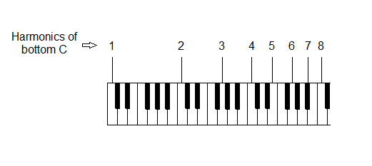
Figure 2. A harmonic spectrum represented logarithmically across a keyboard
Taking the frequency of bottom C as that of the fundamental or first harmonic, the remainder then lie at the positions shown. An identical pattern of harmonics, in terms of their unequal spacings across the page, would be obtained by choosing any other starting note. As stated already, the frequency difference between each pair of harmonics is the same and equal to the frequency of bottom C, or whatever other starting note was used. However the gradually-reducing spacing seen between pairs of harmonics is logarithmic, just as it is in the spectrum plot of Figure 1, because keyboards represent frequencies logarithmically to mirror the processing performed by the ear. (Apart from the octaves, the frequency correspondences between all the other harmonics and notes on the keyboard are not exact, at least in Equal Temperament tuning. This is because of the coarse frequency representation afforded by only having twelve semitones to the octave).
An interesting point is that the pattern of harmonics, when drawn on a logarithmic frequency axis as above, is independent of absolute frequency (the frequency of the fundamental or starting note). This differs from a linear representation, in which the harmonic separation varies depending on the fundamental frequency or pitch of the pipe. Thus our ears might capitalise on this simplification in the pattern processing taking place in the brain.
Thus the spectrum in Figure 1 is a log-log plot in which the numbers on both axes are represented logarithmically to match the logarithmic processing of amplitude and frequency used by the ear and brain. Note how the the harmonics jump up and down capriciously in amplitude as pointed out earlier. This awkward behaviour might not cause too many difficulties if it actually meant something and if it existed for all the pipes in this diapason rank, but in fact it does not. This can be illustrated merely by looking at the spectrum of an adjacent pipe, middle F. Figure 3 shows its corresponding harmonic retinue, plotted together with that for the F sharp pipe we have just been discussing. In this case a linear rather than logarithmic frequency scale was used to prevent the plot becoming visually confused towards the high frequency end of the axis.
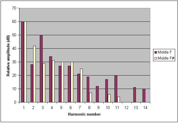
Figure 3. Spectra of two adjacent Open Diapason pipes
(middle F and F#, Walker, 1858)
Both harmonic series were normalised independently to the levels of their first harmonics, so the fact that they both have the same starting amplitude of 60 dB is of no consequence. Beyond this, however, there is virtually no correspondence at all between the two spectra other than their fundamentals have the highest relative amplitudes in both cases. Even the numbers of harmonics are not the same, the F pipe having 14 and the F sharp one only 11. Nor is there scarcely any discernible association between the amplitudes of corresponding harmonics. For instance, the second harmonic of F sharp is stronger than that of F by about 14 dB. This is a factor of five in amplitude. Yet in the case of the adjacent third harmonic the situation reverses - here the amplitude of F is far stronger than F sharp by 21 dB, a factor of over eleven! Perhaps the only slight feature of note is that the data for harmonics 5 and 6 are the same, though these are rather weak at only 1/32nd the amplitude of the fundamentals. So it is unlikely the ear latches exclusively onto these in its search to decide whether the two pipes sound similar.
It should be pointed out that the erratic appearance of these two spectra is not solely a characteristic of the pipes themselves. When sounding in an anechoic chamber or in near-anechoic conditions out of doors, pipe spectra often exhibit smoother envelopes. Thus the effect of the room containing the pipework is partly responsible for augmenting the inconsistencies just discussed. This is because of the multiple standing waves set up at each harmonic frequency due to reflections at the room boundaries, and they result in unpredictable reinforcement or attenuation of the directly-radiated harmonics at the listening position. We do not often encounter organs outdoors or in anechoic chambers, but because our ears have obviously overcome the problems caused by room acoustics because they can somehow 'listen through' to the original sounds, we should like to understand how they do it.
Harmonic Groups
Brains are continually on the lookout for patterns contained within the torrent of data coming in from the senses, and it surely must be the case that the simpler the pattern, the better. Why would they devote processing power to recognising an overly-complex pattern when comparable information could be derived from a simpler one? In what follows we shall see how very simple patterns can be extracted from the confused jumble of data in an organ pipe spectrum.
Depending only on their amplitudes, the harmonics in diapason pipe spectra can be divided into two groups, and this also applies to flute, string and reed stops. I have come to this conclusion having studied them probably for as long as anybody (some forty years). Put simply, the two groups contain those harmonics which are prominent and of high amplitude, and those which are not. Nevertheless both groups are important in forming the tone of the pipe. This grouping can be observed in the Open Diapason spectra in Figures 1 and 3 which have already been discussed. Both spectra have a few strong low order harmonics, meaning the fundamental and some of those close to it, followed by a trailing retinue of higher order harmonics with lower amplitudes. Although one cannot be too dogmatic because one comes across 'rogue' spectra occasionally, a spectrum level about 30 dB below that of the strongest harmonic (which is not always the fundamental) is a useful value to delineate the boundary between the two groups, at least in these examples. Minus 30 dB means the amplitude has fallen by a factor of 32 below that of the strongest harmonic, an appreciable amount. Thus the two spectra in Figure 3 have between 4 and 6 harmonics in the high amplitude group defined in this way, with the remainder falling into the second.
It is an important and happy coincidence that the low order early harmonics, those in the high amplitude group, are those which a pipe voicer can adjust almost individually to some extent. The adverb 'almost' is necessary because voicing adjustments affect all harmonics to some degree. Nevertheless, it is routine practice to adjust the 'brightness' of a diapason pipe by modifying the strength of the second harmonic relative to the first (the fundamental)
[2]. This parameter is strongly influenced by mouth height (the cut-up in organ building terminology) as well as certain other adjustments available to the voicer
[3]. On the other hand, the high order harmonics with lower amplitudes cannot be adjusted individually. Not only are there too many of them crowded increasingly close in relation to their frequencies, but they are too weak to perceive individually. Thus it is as a cluster, rather than as individuals in isolation, that these harmonics contribute enough acoustic power to be important to organ pipe tone. This provides additional justification for separating a spectrum into these two groups of harmonics. In the case of flue pipes, the group of high order harmonics have amplitudes which are a strong function of pipe dimensions, and in particular its cross-sectional area relative to its length (its scale). Pipe scale also affects the rate at which the high order harmonic tail falls off
[4].
Trendline
Analysis
The two groups of harmonics mentioned above are shown in Figure 4 for the same middle F sharp pipe discussed already. Group 1 brackets the first four low order harmonics of relatively high amplitude and Group 2 brackets the remaining high order harmonics having lower amplitudes.
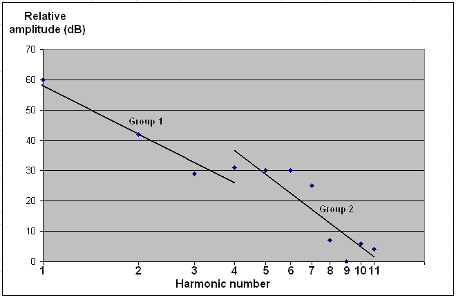
Figure 4. Trendlines and spectral groups for an Open Diapason pipe
(middle F#, Walker, 1858)
Also shown in this plot are two trendlines corresponding to the two groups. Each line was fitted to its group of harmonics using a standard least-squares fitting procedure. The two lines do not have the same slope, nor do they intersect at a point which has any physical or subjective meaning as far as is known at this time. Thus they are apparently disjoint line segments, but this does not matter for present purposes. However the breakpoint between the lines, the point at which the second takes over from the first, occurs at a relative amplitude level about 30 dB down on the fundamental, and near the 4th harmonic. These characteristics seemed to 'drop out' naturally from the spectrum, and they confirm the remarks made previously about the approximate amplitude and frequency values which delineate the two spectral groups.
Trendlines are about the nearest one can get to a spectral envelope of organ
pipe sounds. Spectral envelopes are smooth curves which show how the
harmonic amplitudes vary across a spectrum and they are used widely in fields
such as speech processing and analysis. However they cannot be used, in
fact an 'envelope' as conventionally understood has no meaning, when the spectra
are as ragged as they often are for organ pipe sounds. The harmonics in
Group 2 in Figure 4 illustrate this.
Using the digital technique of additive synthesis it is possible to create an entirely artificial diapason tone using only these two
trendlines. Instead of using the actual harmonic amplitudes represented by the blue dots in Figure 4, new ones are derived by using the trendline values at each of the 11 harmonic positions along the horizontal axis. Although the synthetic diapason does not sound exactly like the real one, it is nevertheless very close and it certainly generates a respectable Open Diapason tone. Crucially, the two real F and F sharp pipes we have been discussing do not sound exactly the same either. The point is that the ear (at least, mine) accepts all three tones, two of them real and the third synthetic, as belonging to the same diapason rank. Therefore we seem to have arrived at a means of reducing the confusing welter of data in the real
spectrum to a much simpler generic form using two trendlines, the generic form nonetheless retaining the essentials of the sound of this diapason
stop which satisfies the ear.
These observations are potentially important because they suggest that the brain might extract 'best-fit' straight line features from an acoustic spectrum to decide which type of organ pipe - flute, diapason, string or reed - it represents.
It might also explain how the ear is so tolerant of the scatter among the harmonic amplitudes of aurally-similar pipes belonging to the same rank which is so frequently encountered. Changes in the random scatter affecting the group of harmonics to which a linear trendline is fitted will usually not materially affect the parameters of the line itself (its gradient and intercept on the axes). This because, while the amplitude of a certain harmonic might increase from one pipe to another, that of its neigbour or another elsewhere might decrease. This would necessarily happen if the changes were indeed random, otherwise they would be systematic and related to some deterministic cause which could be identified. Moreover, the extraction of line features by brains has been accepted for some decades as playing a major role in visual pattern recognition and scene analysis
[5]. In addition, some neurophysiologists incline to an economic view of brain architecture in which similar neural circuitry could be used for performing quite different functions
[6]. Therefore it is tempting to suggest that extraction of linear trendline features in organ pipe spectra might indeed take place in the
brain as it does for visual processing.
It could be said that an acoustic spectrum is a 2-dimensional picture, and indeed it has been treated as such in this article and widely elsewhere. In fact it is so common a practice that it never attracts a moment's thought.
The spectrum files on this web page are picture files. So if the data arriving from the inner ear were to be projected within the brain in a similar way to the 2-D mapping of pictures in the visual cortex, then it is no great extrapolation to imagine that similar pattern processing (such as extraction of line features) might be used in both cases. It is known that frequency information is organised tonotopically (in frequency order) within the auditory cortex, and a similar arrangement might also exist for amplitude information. If this is so, then a complete spectrum could be represented as a picture in the brain, and picture processing techniques
such as the detection of line features could then be applied to it before we experience a conscious perception of the sound it represents.
Another important observation is that the ability to use the simplest form of trendline in this analysis, a straight line, was only possible because a log-log plot was used to represent the spectrum in amplitude and frequency. This mirrors the logarithmic processing of amplitude and frequency used by the brain. It is easy to demonstrate that, if a linear rather than logarithmic frequency scale had been used, the best-fit trendlines would be more complex in that they would be curved. Thus the use of linear trendlines for aural processing is an appealing hypothesis in view of their simplicity and the fact that brains are known to extract linear features from other types of sensory data.
The frequency spectra of Flute
pipes
Having covered diapasons in detail, we can now discuss the other classes of organ tone more quickly. So now we turn to organ flutes. These have far fewer harmonics than any other type of organ pipe, and an example with only six harmonics (a typical figure) is shown in Figure 5. This represents a Stopped Diapason speaking middle F sharp on an 8 foot stop from the same Walker organ at Ponsbourne considered above.
Figure 5. Spectrum of a Stopped Diapason pipe
(middle F#, Walker, 1858)
Contrary to what its name implies, this pipe is not a diapason at all but one with a particular type of flute tone, the particularity deriving from the pronounced amplitude differences between the odd-numbered harmonics and the even ones. This arises mainly because the top of the pipe is closed by a stopper. The consequential suppression of the even harmonics endows such pipes with a pronounced hollow, 'woody' tone. Nevertheless, even in open flute pipes without a stopper, the even-numbered harmonics are usually of lower amplitudes than those in diapasons and strings, this behaviour resulting from deliberate voicing adjustments applied to the pipe mouth. All of these factors are described in detail in references
[7] and [8].
Thus it is quite easy to identify two linear trendlines in the spectra of most flute pipes which correspond to the even and odd harmonic series, as drawn in the figure above. Note that it is not possible to define the harmonic groups and trendlines in exactly the way it was done for the diapason spectrum discussed earlier, because there are insufficient harmonics here. There is no equivalent of an extended tail of harmonics with decreasing amplitudes in this case, for example. But, and as for the diapason, a wide range of generic but nonetheless realistic flute tones can be synthesised using only these two trendlines because the ear is extremely sensitive to the relative proportions of odd to even harmonics in musical tones. Only four adjustable parameters are required to realise this range of flute timbres because a straight line is fully defined using just two numbers- these are the slope of the line and its intercept on the vertical axis. This simplicity suggests the brain might reduce the presented spectrum to its essentials in this way, perhaps using the 'picture processing' mechanism hypothesised previously. However, note again that the spectrum must be plotted using logarithmic scales on both axes otherwise the trendlines are not straight but curved. In this case they are less readily identified by eye as well.
The frequency spectra of String
pipes
String toned pipes have more, often far more, harmonics than any other type of pipe speaking the same
pitch. This is illustrated in Figure 6 which shows the spectrum of a keen-toned string pipe on the Rushworth and Dreaper organ at Malvern Priory, England.
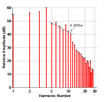
Figure 6. Spectrum of a Viol d'Orchestre pipe
(middle F#, Rushworth & Dreaper, 1927)
Only about 30 harmonics are shown to prevent the plot becoming too cluttered towards the higher frequencies, but it is apparent that it could otherwise have been continued because they show no sign of suddenly dropping towards the zero line. This attribute arises because string pipes, at least the keen-toned ones, are much narrower than diapasons and flutes, and the consequences this has for their tone are explained in references
[7] and [9]. Uniquely among the flue pipes,
such strings also have a series of low order harmonics whose amplitudes rise to a maximum around the fourth, as in this case. Thus the strongest harmonic is not usually the fundamental as in the case of flutes and most diapasons.
It is not difficult to identify three groups of harmonics in this spectrum. These are the rising series up to the fourth, a descending group with a slope of -6 dB/octave and a third decreasing at a greater rate. However it is possible in many cases to include all harmonics after the strongest
(the fourth in this instance) in a single group, thereby reducing the number of spectral groups to two as with the diapason. As with the diapason and flute spectra, each group can be approximated by a
trendline. Only the -6 dB/octave line has been drawn in the figure though the other two can be visualised readily.
As with diapasons and flutes, synthesis of a convincing string tone can be achieved using the trend line data alone. In this case it would represent a particularly large reduction in the amount of information to be processed by the brain. The amplitudes of more than 30 harmonics would be replaced by the slopes and relative positions of just three (or even possibly two)
trendlines. This is an example of dimensionality reduction, which is important in this context for two reasons. Firstly it reduces the load thrown onto the pattern processor, in this case the brain. Secondly, it enhances the generality or range of patterns which the processor can identify as belonging to the same class even when the individual patterns are noisy. We have seen already how organ pipe spectra are corrupted by noise in the form of random variations in the harmonic amplitudes from one pipe to another.
The frequency spectra of Reed
pipes
The spectrum of a reed
pipe is shown in Figure 7, representing middle F sharp on the Swell Organ Trumpet at Malvern Priory, England
(Rushworth & Dreaper, 1927).
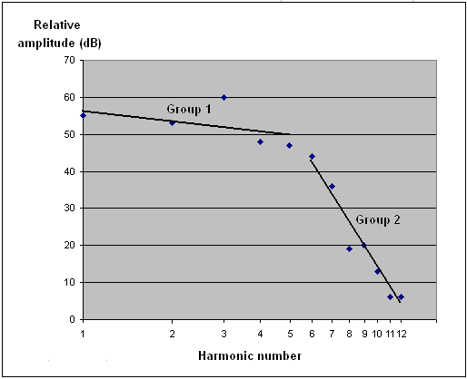
Figure 7. Trendlines and spectral groups for a Trumpet pipe
(middle F#, Rushworth & Dreaper, 1927)
As before, the harmonics fall naturally into two groups. Group 1 includes harmonics 1 to 5 and Group 2 the remainder. Trendlines are fitted to each group. Superficially, the spectrum, groups and trendlines resemble those of the Open Diapason (Figure 4), but there are in fact significant numerical differences which account for the very different tone of the two types of pipe. Firstly, the slope of the line corresponding to Group 1 is more nearly horizontal than for the diapason, and for many reed stops it is indeed horizontal or it even slopes slightly upwards. This illustrates the way that the low order harmonics of a reed are maintained at higher powers compared with those of flue pipes. By contrast, harmonics beyond the fifth then fall away more rapidly than for the diapason, thus the Group 2 trendline has a steeper slope in this case.
It is therefore remarkable that two quite different tones can be approximated by the same dual trendline model with only four independent parameters, these being the slopes and vertical axis intercepts of the two lines.
A model with only a handful of parameters which seems to encode the essential auditory features of two very different organ pipes with many harmonics - diapasons and reeds - yet again provides food for thought. Once more it makes one wonder whether the pattern processing taking place in the brain does indeed latch onto these simple line features in the spectra.
Their high power harmonic retinue results in an interesting psycho-acoustic feature of many reed pipes. This is that the fundamental or first
harmonic can sometimes be much weaker than it is in Figure 7, indeed occasionally it can be almost absent.
It can also be removed deliberately using digital techniques. Yet in some (but
not all) of these cases the ear nevertheless has no difficulty assigning the correct musical pitch to the pipe, pitch being defined by the frequency of the weak or missing fundamental. This phenomenon is investigated in detail in reference
[10] (see the section entitled The Mystery of the Missing
Fundamental) with the help of some audio examples. On the
other hand, the strong third harmonic here is noticeable in the tone, and
adjusting its amplitude in a digital reconstruction results in clearly audible
differences. So the third harmonic certainly could not
be removed. However it is difficult to say whether this particularly
strong harmonic was a
defining characteristic of this particular pipe or whether it was merely an
artefact due to augmentation by standing waves in the church when the sound was
recorded.
Concluding
Remarks
This
article has shown that the four classes of organ pipe tone - flutes, diapasons
(or principals), strings and reeds - have frequency spectra which, as often as
not, are characterised by significant amplitude scatter which obscures their
systematic structure. In this sense they are noisy, with the noise having
no apparent correlation between musically-adjacent pipes a semitone apart.
Some of the scatter arises owing to reflections at the boundaries of the room
housing the organ, giving rise to a different pattern of standing waves for each
radiated harmonic which attenuates or augments its amplitude in an unpredictable
manner at the listening position. It is therefore remarkable that
our ears have little difficulty in deciding that the sounds from a given rank of
pipes belong to the same stop on an organ. However spectral groupings of
harmonics have been identified in most if not all of the many spectra analysed over some forty years of research, and each can be associated with a
linear trendline fitted to the harmonics of its group. Using the real discrete
inverse Fourier transform to perform additive synthesis, it has been found that
the subjective tone quality or timbre of a pipe is little changed when it is
reconstructed from its trendline values rather than from its actual harmonic
amplitudes.
In any case, such differences as do exist between the actual sound of a pipe and
its reconstruction are often eclipsed by those occurring naturally
between adjacent pipes owing to the gross variations in their spectra. In most
cases only two groups seem to occur in each spectrum, and therefore only two trendlines are required.
This
finding might be significant in aural perception because it is a means of reducing the confusing welter of data in
real spectra to a much simpler generic form using two trendlines, the generic form nonetheless retaining the essentials of the sound of
an organ pipe which satisfies the ear. Because the ear and brain process
both amplitude and frequency logarithmically, the trendlines themselves on a similar log-log spectrum plot take the simplest possible form,
namely straight lines rather than curves. This being so, each trendline is
defined using
only two parameters - its slope and its intercept on the amplitude axis.
Thus a noisy spectrum with an arbitrary number of harmonics can be reduced to
just four numbers which nevertheless seem to encode the essential subjective features
of the spectrum. This represents a considerable dimensionality reduction
in a spectrum with many harmonics which has implications for acoustic pattern
recognition whether implemented by brains or machines.
It
is well-established that brains extract linear (straight line) features when
processing visual sensory inputs, and it is therefore possible that similar neural
mechanisms might operate when processing the auditory sensory data arriving from
the inner ear. An amplitude-frequency spectrum is merely a 'picture' which
must be projected within the auditory cortex in some way, and it is conceivable
that linear features within it - such as the trendlines discussed here -
are extracted as part of the acoustic pattern recognition processes in the
brain. There would seem to be implications for the mechanisms of musical perception in these
suggestions.
Since this article was posted several others have appeared which describe some
practical applications of trendlines in tonal analysis and music synthesis [11].
Notes and References
1. Two articles elsewhere on the site describe how flue and reed pipes emit sound:
How the flue pipe speaks
How the reed pipe speaks
Building on these, four other articles are devoted to the main classes of organ tone:
The Tonal Structure of Organ Flutes
The Tonal Structure of Organ Principals
The Tonal Structure of Organ Strings
The Tonal Structure of Organ Reeds
Like the present article, an earlier one also investigated some aspects of how organ tones
might be perceived:
The Aural Perception of Organ Tones
2. Broadly speaking, principals in continental Europe by builders such as Gottfried Silbermann in the 18th century had stronger second harmonics (relative to the first) than did those found in Britain in the 19th century and into the 20th. This partly accounts for their brighter and more zestful tones compared to the more subdued sounds of British diapasons. A detailed study of this and other characteristics, including some audio examples, can be found in the article
The Tonal Structure of Organ Principals .
The
application of trendline methods to reveal this and other differences between
baroque and romantic principal stops is described in Objective
differences between the sounds of baroque and romantic principal stops .
3. Voicing adjustments and their effect on the sounds of flue pipes are described in detail in the article
The Tonal Structure of Organ Strings in the section entitled
The Physics of Voicing.
4. The effect of flue pipe scale (cross-sectional area relative to length) on the total number of harmonics, and hence on the number of high order harmonics of relatively low amplitude occupying the high frequency tail of the spectrum, is discussed in the article
How the flue pipe speaks . The narrower the pipe, the more harmonics it emits. Keen-toned string pipes often have more harmonics than reeds of the same musical pitch, and strings are discussed in the article
The Tonal Structure of Organ Strings.
The
application of trendline methods to reveal these and other differences between
baroque and romantic principal stops is described in Objective
differences between the sounds of baroque and romantic principal stops .
5. "Receptive fields of single neurons in the cat's striate cortex", D H Hubel and T N
Wiesel, Journal of Physiology, 148 (3), p. 574, 1959.
6. William H Calvin drew parallels between brain functions which appear quite different at first sight, such as predicting an optimum ballistic trajectory to hit prey with a spear and the syntactical analysis required for understanding speech. He therefore proposed similar brain mechanisms to perform these functions using a 'Darwin Machine' model. See:
"How Brains Think", William H Calvin, Weidenfield & Nicolson, London 1996.
7. See How the flue pipe speaks
8. See The Tonal Structure of Organ Flutes
9. See The Tonal Structure of Organ Strings
10. See The Tonal Structure of Organ Reeds
11.
Since this article was posted several others have appeared which describe some
practical applications of spectral trendlines in tonal analysis and music synthesis:
The Effect of Organ Pipe Scales on their Harmonic Spectra
- shows how trendlines can reveal the aural effects of organ pipe scaling laws
Trendline
Synthesis - a new music synthesis technique - the application of
trendline techniques to the digital synthesis of musical tones
Scaling
synthetic samples across the key compass - how trendlines lead to an
intuitive way of scaling (varying the timbre of) digital sound samples across
the keyboard
A
technique for simplifying parameter estimation in synthesised organ pipe
sounds - shows how spectral trendlines offer a streamlined
way of voicing digital organs
Objective
differences between the sounds of baroque and romantic principal stops - using
trendlines to reveal timbral variations between different stops of the same
family