


|
|
|
Physical Modelling in Digital Organs
by Colin Pykett
Posted: 25 March 2009 Last revised: 9 April 2012 Copyright © C E Pykett
Abstract. Synthesisers using physical modelling have been commercially available for about 15 years whereas digital organs using other synthesis methods have been around for about 40. However it is only recently that physical modelling is appearing in digital organs. This article explains physical modelling in simple terms by describing the commonly used technique of waveguide synthesis applied to organ pipes. In addition it covers the wind system and acoustic coupling models which are also necessary for successful modelling of the organ. However, because these can also be incorporated in conventional digital organs using sampled sounds or additive synthesis, these instruments have been able to simulate pipes to a high degree of realism for some years.
Although manufacturers continue to emphasise the small variations which occur in pipe speech, these are negligible compared to the vast range of expression which any orchestral instrument is capable of. The corresponding effects on the simulated pipe sounds are limited to small variations in pitch and amplitude, which can both be rendered by modern sound sampling and additive synthesis techniques. Although it is not disputed that physical modelling is capable, in principle, of simulating pipe organs to a high degree of fidelity, it seems reasonable to view it as another way to do the job rather than as an intrinsically better one.
Contents (click
on the heading to access the desired section)
Physical modelling in simple terms Physical modelling in more detail
Waveguide model of a flue pipe
Factors
affecting “live” pipe speech
Electrical modelling analogies
Each time an organ pipe speaks it always sounds more or less the same. Although some maintain that a pipe never speaks the same way twice, it is difficult for them to argue that the differences are other than small. Thus it could be said that organ pipes have fewer musical and acoustical degrees of freedom than most other instruments, but those which do exist admittedly might endow the pipes with a “live” character. Examples are the small variations in their attack and release transients sometimes experienced with mechanical actions, or the way pipes react to the presence of others in that their tuning can be “pulled” by those already speaking nearby. Or an intrinsic unsteadiness in their wind supply can sometimes be modulated by how many stops are drawn and the rhythmic nature of the music being played (often called “live winding”). All these individual characteristics vary from pipe to pipe and from stop to stop. On the whole, pipe organ builders appear to regard them as imperfections and they strive to suppress them, whereas digital organ makers strive to emulate them! Nevertheless, and in contrast to other wind instruments, the organ remains inexpressive. Even with the “imperfections” just mentioned, any expression that can be coaxed from it by the performer is almost non-existent and entombed within the virtually invariant sound of its pipes. At the other extreme an oboe, for instance, forms an integrated living whole with its player, who can instantaneously modulate its tuning, loudness and tone quality over a wide range as well as impose vibrato with characteristics of unbounded subtlety. As I play both instruments I can speak with some experience. Similar attributes apply to all other woodwind, brass and stringed instruments. By comparison the pipes of an organ sound virtually the same each time they speak. Although there might be differences from one time to the next, it is difficult to argue that they are other than second order effects when set against the expressive capability of their orchestral counterparts. In many organs the small variations in speech which do exist are imperceptible in reality even to the player, maybe at a detached console and controlling by means of an electric action thousands of distant pipes whose sounds become immediately submerged in the ambient acoustic swirl of the building. To an audience, additionally immersed in its own background noise due to fidgets, coughs, nose-blowing, throat clearing and furtive manipulation of candy wrappers, the differences are entirely irrelevant. Only with a top-rank player on a small organ with a mechanical action in a dry acoustic and a small, attentive audience will the minute nuances of pipe speech have a chance of enlivening the performance in the minds of the listeners. So why do digital organ makers raise the profile of the tiniest details of pipe speech to the extent they do? The answer to this question is not trivial because it requires an examination of how digital organ technology continues to evolve. Since the introduction of a new form of technology will have involved a firm in significant investment over some years, one needs to ask why they took the associated risks when most digital organs are now pretty good to start with and have been so for many years. The answer to this question obviously cannot be glib if it is to be convincing because a sensible firm will not inflate its cost base to fund additional R&D without good reason. Therefore this article expands this thread by looking in more detail at the latest technology now emerging in digital organs – physical modelling. Physical modelling in simple terms Before describing what is meant by the term physical modelling, it is useful to briefly review the two other main techniques used in music synthesisers in general and digital organs in particular. The first is synthesis using sound samples, and the second is additive synthesis operating on tables of harmonic amplitudes which define the frequency spectrum rather than the time waveform of the sound. Digital organs using sampled sounds form the majority in use today. The sounds of actual organ pipes are recorded and then stored as digital waveforms in the computer memory of the organ. The alternate method - additive synthesis - means that the harmonic strengths of the waveforms are stored rather than the waveforms themselves. In this case the sounds of the organ are derived by a process called additive synthesis in which the harmonics are first added together before emerging from the loudspeakers as a complete waveform. In
both these cases the computer system within the organ re-creates these
predefined sounds without any consideration of how real organ pipes actually
work. This means that most
conventional digital organs have no internal representation of acoustical
physics beyond the binary numbers which describe the waveforms or the frequency
spectra. Until the pipe waveforms
or tables of harmonics are loaded into it at the factory, a conventional digital
organ cannot make the merest squeak. At
that stage it is analogous to a pipe organ without any pipes sitting on its
soundboards. With physical
modelling on the other hand, sounds are not re-created directly from predefined
information – they are created and controlled from scratch by mathematical
models that ultimately produce
those sounds. Although at first
sight the difference might seem academic, it is vital that one understands what
it means if one is to understand what physical modelling is about.
Thus one is now defining a model of an actual organ pipe in the
form of equations, and one programs the equations into the computer rather than
putting in the waveform of the pipe or its harmonic structure.
Then, when you key a note, you are setting the model running and it will
duly calculate in real time the waveform of the pipe.
The waveform does not exist until this point, just as the sound of a real
pipe does not exist until you admit wind to it when playing a pipe organ. What
advantages does this confer? The
answer to this question is easy if the object of the exercise is to model the
sound of a piano, for instance, but less clear for a pipe organ.
This distinction between the organ and other instruments will crop up
time and again in this article to the extent that it becomes awkward.
It is a consequence of the relatively invariant nature of organ pipe
sounds already discussed. But for a
piano, everyone knows that the harder you hit the key the louder the sound.
Most people also realise that the tone quality varies as well, as does
the attack transient and the decay characteristics. The differences are not only subtle but important, thus
simulating a piano properly is difficult and expensive.
With sampled sound synthesisers it is often done by having several stored
waveforms available for each note, each of which was recorded on a real piano by
pressing the corresponding key at a different speed.
The waveform actually used is then selected on the basis of key velocity
when the digital piano is played. However
this is a rather crude approximation to reality. It means that the sound of a digital piano will suddenly
change when the key velocity moves from one to another of a few velocity
regions, a characteristic quite foreign to the real instrument. But by using physical modelling this problem can be
eliminated. One sets up a
mathematical model of the piano action for a key, its string(s) and the
soundboard, in which one of the input variables is key velocity.
Then the computer is able to calculate the sound waveform corresponding
to any velocity, not just the few for which sound samples were recorded
in the sampled sound approach [7].
This is obviously preferable by far to the older synthesis methods, and
similar advantages apply when simulating instruments such as woodwinds, brass or
strings. But what advantages might accrue if physical modelling was used to simulate an organ? Because of the almost invariant nature of pipe sounds which can already be reproduced more or less exactly by current digital organs, especially those using sampled sounds, physical modelling cannot really offer the major advantage just outlined for the piano. It could certainly simulate the relatively minor variations in pipe speech discussed already, but it will be shown later that most if not all of these minor variations can already be simulated using the traditional methods of sampling or additive synthesis. Interest in physical modelling began to accelerate around the early 1970’s when the work of physicists including the late Arthur Benade showed that instruments such as the clarinet could be successfully modelled to a high degree of fidelity. Among many other things, he and others developed equations which modelled the subtle acoustic mechanisms of the tone holes in this and other wind instruments. However the work existed more as a portfolio of elegant concepts for some years rather than finding immediate commercial applications in music synthesis. This was because computer technology was neither cheap enough nor unable to work at the necessary speed to enable successful real time operation, although the models continued to be refined and validated at various universities. Coincidentally, these early concepts arose at about the time the first digital organs by Allen appeared, though they did not use physical modelling of course. These early instruments used stored waveforms and they monopolised the digital organ field until the associated patents began to expire in the 1990’s. At that point the floodgates opened and many other manufacturers, hitherto forced to use analogue methods, were suddenly able to market instruments using sampled sound technology. Additive synthesis for organs had arisen at Bradford university in the UK in the 1980’s, when the strength of the existing stored-waveform patents was still preventing other manufacturers from using the sampled sound technique. But because additive synthesis does not require the storage of sound samples it was able to sidestep them. So if physical modelling has existed as long as the other two methods, why has it not appeared before on the digital organ scene? The main reason was mentioned above in that practical (i.e. real time) implementations of existing mathematical models did not become economic or feasible until digital processing hardware of sufficient power started to appear in the late 1980’s. By “power” is meant microprocessor systems of sufficient speed with memories of sufficient capacity, all readily available at sufficiently low cost.
Physical modelling applied to digital organs was introduced by Viscount in about 2006. Some software synthesisers also use physical modelling which can be used to simulate organ sounds as well as other musical instruments. As far as this article is concerned it is important to note that it relates to the body of techniques constituting physical modelling in general rather than the offerings of any manufacturer in particular. Currently
(2009) many of the early patents for physical modelling appear to be owned by
Stanford university in the USA and Yamaha, who entered into a contractual
arrangement in about 1989. An early
offspring of this union was the first commercial synthesiser to use physical
modelling brought out by Yamaha in 1994, which again was a long time after
digital organs first appeared. So
it is also possible that the delayed appearance of physical modelling in the
restricted field of digital organs might be related to the expiry of some
of the early patents, though currently it is difficult to be certain on this
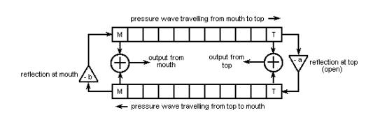
point. Physical modelling in more detail This section is optional and can be skipped. If you are not particularly interested in learning more about physical modelling at this time you can move on to subsequent sections of this article without losing overall comprehension of what it is about. The field of physical modelling for music synthesisers is now vast and highly technical, having been spurred on by the prospect and actuality of lucrative commercial returns for many years. Much of the theory and enabling technology is described at various levels of detail in many places on the Internet so it is unnecessary to repeat or summarise it here. The Wikipedia entry dealing with the subject [2] might be a useful starting point. However there is little relating specifically to modelling the pipe organ, therefore one of the most common techniques, waveguide synthesis, will now be described at a relatively simple level without resorting to mathematics. Note that the inclusion of waveguide synthesis here does not imply that commercial digital organs will necessarily use this method as there are also several others in widespread use. It is included as a generic technique for purposes of illustration only. The physics of sound production in flue pipes and reed pipes is discussed in detail elsewhere on this website in references [3] and [4] respectively. Waveguide synthesis uses these physical principles to construct the sound wave which would be emitted by a pipe when the appropriate key is pressed and the appropriate stop drawn in a digital organ. The term “waveguide” first arose during the second world war in circumstances far removed from digital musical instruments. It denoted a structure used to contain and guide radio waves at the extremely high microwave frequencies used by the then-novel radar systems which were being intensively developed, and they consisted of nothing more than lengths of tubing with rectangular or circular cross-sections. Pretty much like organ pipes in fact, which can also be looked at in terms of waveguides but for sound waves rather than radio waves. The mathematics can get fearsomely complicated for both cases if you give it free rein, but fortunately we can get some idea of how waveguides work by ignoring it here. Waveguide model of a flue pipe Reference [3] shows that there are two sets of travelling sound waves in a flue pipe, one set travelling up the pipe from the mouth to the top, and the other travelling down in the reverse direction owing to the reflection at the top. They exist simultaneously once the pipe has settled down to stable speech, therefore at any point inside the pipe the net sound pressure is the sum of both the upward-travelling wave and the downward-travelling one. In this situation we get so-called standing waves, and many readers will be familiar with diagrams of the air pressure nodes (pressure minima) and antinodes (pressure maxima) at the various harmonic frequencies which exist in a flue pipe. More detail about standing waves and other physical aspects of a wide range of flue stops can be found in the articles elsewhere on this site which discuss the various types of organ flute [5] and the various types of principal [6]. To model the standing wave in a flue pipe it is convenient to visualise two waveguides, one dealing only with the upward-travelling wave from mouth to top and the other dealing only with the downward-travelling wave from top to mouth. This arrangement is sketched in Figure 1 for an open pipe, one which has no stopper at the top. Each waveguide is represented by the horizontal array of small boxes or compartments. Each compartment holds the most recent result of a pressure calculation for that point inside the pipe. The mouth of the pipe is represented by the two left-most compartments labelled M, and its top is represented by the two compartments labelled T.
Figure 1. Waveguide synthesis – open flue pipe An open flue pipe emits sound both from its mouth and its top, so to calculate these outputs we need to add the sound pressures of the two travelling waves at these points, shown in the diagram by the adders connected to the ‘M’ and ‘T’ boxes. A further step, not shown, is then necessary to calculate the overall sound emitted into the auditorium by adding the “mouth” and “top” outputs together with the correct proportions and phases. These will be affected to some extent by the spatial position of each pipe in the auditorium and could therefore differ for each one. The model is started when we in effect admit wind to the pipe by pressing the associated key with the associated stop drawn. Just prior to that the modelled air pressure values in all the compartments will be the same and equal to atmospheric pressure. Admitting wind means there is a sudden increase in air pressure in the ‘M’ compartment at the left of the top waveguide, and this also appears at the output of the adder connected to the compartment. In turn this means that a sound wave will begin to form at the mouth of the simulated pipe, and it is the beginning of the attack transient of the pipe being modelled. In the digital organ it is applied to the loudspeaker system of the instrument as a corresponding voltage. A short time afterwards the model propagates the pressure impulse into the next compartment, and it is added to the existing pressure value already there (atmospheric pressure in this case). The time interval involved is short and it will depend on various factors, including the fundamental frequency or musical pitch of the pipe. Typically it will be measured in a few tens of microseconds. The pressure increment which is added into the new compartment is not the same as that which was originally added to compartment ‘M’ because as the pressure pulse travels along the waveguide, or up the simulated pipe, it must gradually lose energy as it would do in reality. Therefore the propagated air pressure increment must be reduced by a small amount. Simultaneously the value of air pressure in ‘M’ is reduced because some of its energy has now been transferred into the adjacent compartment. In the same way, over a succession of short time intervals, the model successively propagates the air pressure impulse along the waveguide to the right until it arrives at compartment ‘T’, the top of the pipe. At this point it is immediately transferred into the ‘T’ compartment of the lower waveguide via the triangular symbol (a multiplier) which multiplies the pressure by -a. The negative sign here means that the phase of the pressure impulse is reversed in that it now becomes a rarefaction rather than a compression, whose value is now subtracted from the atmospheric pressure in the lower waveguide rather than being added to it as before. The phase reversal is necessary because this is what happens at the top of an open pipe when the upwards-travelling wave is reflected back into the pipe [3]. The value of a must be less than one, otherwise there would be no output from the adder connected to the two ‘T’ compartments, and therefore there would be no sound emitted from the open top of the pipe. The new negative pressure increment in ‘T’ now propagates along the lower waveguide towards the left until it reaches the ‘M’ compartment which is the mouth of the pipe. This propagation represents the reflected wave moving back down the pipe. When it reaches the mouth its phase is reversed again because of the minus sign in the multiplier containing the number -b, converting it back to a positive pressure impulse. Unlike the situation at the top of the pipe, it is not reduced in amplitude however because it receives a kick of energy from the incoming air at the mouth [3]. Rather, it is increased by an amount equal to the total losses experienced by the propagating impulse in order that the pipe will oscillate continuously. Therefore, unlike a, the value of b is greater than one. This process consisting of up-and-down travelling waves continues indefinitely as long as the key is held down. An interesting feature of this model, highly simplified though it might be, is that it takes a number of complete up-and-down cycles before the sounds emitted at the mouth and top of the pipe stabilise. This reflects the attack transient which occurs in real organ pipes. However this is indeed a very simple model and it would not produce a very convincing simulation of a real flue pipe. It is necessary to include many additional features, including the end-corrections at the mouth and top of the pipe and the detailed shape of the initial pressure impulse when the note was keyed. The formation of the air jet by the flue also needs to be carefully modelled, as does the wind noise which accompanies it. All these will depend on the dimensions of the languid, mouth and pipe body and the way the pipe was voiced. However the important point to note is that, if the model is a good one, it is only necessary to provide it with a set of numbers defining factors such as the pipe dimensions, voicing parameters such as nicking and the wind pressure. The model would then calculate for itself the sound emitted by the pipe without having to include explicit additional information about end-corrections, etc. In practice it can be difficult to develop such models, not only because of their theoretical complexity but because it might be impossible for them to run fast enough even on current hardware. Bear in mind that the hardware and software must be able to support many models all running simultaneously, reflecting the situation when many stops might be drawn with many notes keyed. This is no different to the polyphony problem experienced with conventional digital organs using sampled sounds or additive synthesis. If there is insufficient polyphony with any form of synthesis, including physical modelling, then the player will experience missing notes with full combinations of stops and many notes played. To prevent this happening, the model might have to be simplified to the extent that its shortcomings in terms of fidelity of synthesis could become noticeable. It is by no means the case that physical modelling will automatically endow a digital instrument with better fidelity than one using sampled sounds or additive synthesis.
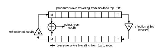
Figure 2. Waveguide synthesis – stopped flue pipe A simple model for a stopped flue pipe is sketched in Figure 2. There are two differences from that for the open pipe case (Figure 1) – firstly no sound is emitted from the top of the pipe so the adder at that point is omitted, and secondly the reflected wave undergoes no phase change when it bounces off the stopper as explained in [3]. Therefore the multiplicand at the top of the pipe is a positive number rather than a negative one. Otherwise the two models work in much the same way. An interesting feature of this model, simple though it might be, is that it will not generate any even-numbered harmonics. This is appropriate for stopped pipes in which the odd harmonics predominate. However the simulated pipe will nevertheless sound artificial when using such a simple model because in practice it is necessary to include the low levels of even harmonics which are present in the sound of a real pipe. A real stopped pipe never suppresses the even harmonics completely. This means the model needs to be considerably more complicated in practice than that shown here. The physics of the organ reed pipe are described in detail elsewhere on this website [4] and, like the flue pipe, it can also be modelled successfully using waveguide methods. There is little room for arguments and excuses here because the clarinet was one of the first instruments to be successfully modelled in detail by workers such as Benade some 40 years ago, and the clarinet is far more complicated than any organ reed pipe. This is because of the many variables characterising the player’s embouchure (the way the reed is controlled via the lips and mouth), the continuously variable blowing pressure and the subtle acoustic mechanism of the tone (finger) holes. Also it operates over a frequency range of several octaves. None of these is present in the organ reed pipe – there is obviously no equivalent of the embouchure, the wind pressure is fixed, there are no tone holes and the pipe emits only a single fundamental frequency. Therefore it is much easier to set up a physical model of an organ reed pipe than a woodwind instrument. There are several major differences between flue and reed pipe models because of the different oscillation mechanisms and the wider range of resonator shapes and sizes in the case of reeds. However physical models of reed pipes will not be discussed further here because the main features of waveguide modelling have already been described above. Factors
affecting “live” pipe speech Earlier in this article the small variations which occur when organ pipes speak were mentioned. We need to discuss them in more detail because, although they can be simulated by physical modelling provided the model is good enough, they can also be simulated by the older methods of sampling and additive synthesis in most cases (again providing the simulations are good enough), and this needs to be pointed out explicitly. The huge number of factors which cause a pipe to sound as it does can be categorised in two ways – those which are constant and do not vary, and those which exhibit small variations. Examples of constant factors are the dimensions of the pipe mouth such as the cut-up (height of the upper lip above the lower). Examples of variable ones are the small variations in wind pressure which occur either randomly due to air turbulence, or (for example) those which occur because of how many other pipes happen to be speaking at the same time. In this article we only need address the variable factors. The fixed ones are irrelevant to whether physical modelling is used or not, because the invariant way they affect the sound of a pipe is reflected equally well by sampling in which the sound of a real pipe can be copied to an arbitrarily high degree of exactness. (This is not quite the case for additive synthesis which does not and cannot exactly copy the time waveform of a pipe; the recorded sound must be processed – transformed from the time domain into the frequency domain - before it can be put into the memory of a digital organ). Returning to variability in speech, the way an organ pipe speaks can only vary from one time to the next because of fluctuations in the wind supply as just mentioned, or because of acoustic coupling between itself and others, or because of the way its valve opens and closes. The latter is only relevant in an organ with mechanical action of course, because with electric and pneumatic actions there are no differences in the valve dynamics each time it opens or closes. Even mechanical actions can only affect the beginning and end of the note, not the sustain (steady state) phase, thus they can only vary the attack and release transients which might be emitted. These will be discussed presently, as will acoustic coupling. However variations in the wind supply affect all phases of pipe speech, and moreover they occur regardless of the type of action. Therefore wind system modelling is an important topic which will now be discussed. Wind pressure affects many aspects of pipe speech, therefore it is necessary to model the dynamics of an organ winding system if pipe sounds are to be accurately simulated. Note that a wind system model is independent of the pipes themselves, therefore it can be used with any form of tonal synthesis, not just physical modelling. In fact it has been applied to a number of commercial digital organs using sampled waveforms for some years, and a number of patents exist which can be consulted for the details. Wind pressure in a pipe organ is supposed to be constant, and in some cases it is. The use of Schwimmer pressure regulators for each soundboard, which use small valves with a rapid response, can result in rock-steady wind to the extent that the regulator has to be thrown out of action if the tremulant is to work! But in other cases there is some unsteadiness in the wind supply – “live winding” - which is either accidental or encouraged. For instance, resonances can occur. Resonance can happen in any system which has both mass and springiness, but it can be controlled (damped) by resistive processes which cause oscillatory energy to be lost through conversion to heat. In a traditional organ winding system there is lots of mass present, including the reservoir (bellows) top board and its loading weights. Even the compressed air itself enclosed in the reservoir, trunking and elsewhere has a surprisingly high density of 1.2 kg/m3 , a substantial figure which is equivalent to about three cans of beans in a large cupboard. Springiness arises from the highly compressible air, and from the coil springs sometimes attached to the reservoir boards. Therefore it is not surprising that wind system resonances are often heard in the form of fluttering or unsteady speech, usually transient rather than continuous. The effect is often most obvious when small high pitched pipes are sounding at the same time as the pedals are playing an independent part, or large bass pipes keyed on the same soundboard can produce the same effect. Resonances can be damped by increasing energy-dissipating resistances in the winding system, such as by attaching dashpots to the reservoir top board. Instabilities can also be reduced by small concussion bellows placed close to the affected soundboard – these smooth out the fluctuations in a similar manner to the large smoothing capacitors used in electronic circuits. Wind sag is a permanent drop in wind pressure while pipes are sounding rather than a transient or oscillatory one, and it is related to the phenomenon of “robbing”. Often it occurs as progressively more stops are drawn on a bar and slider chest because the pallet is too small for the pipework assigned to it. It therefore throttles the wind supply into the groove or channel above it, resulting in a pressure drop which causes the pipes to go noticeably flat. Of course, there are other causes of wind sag which can result from an excessive constriction anywhere in the air supply to the pipes. Sometimes the blower itself cannot supply enough wind to full organ, and this can be manifested if the reservoir collapses while a chord is held at the end of a piece. The sudden drop in pitch which occurs after a second or two is embarrassing and inexcusable. Why anyone would want to model such gross defects is beyond me, but some digital organ devotees apparently do. Other aspects of wind system modelling include detailed attention to the type of valve used to admit air to the pipes (traditional pallet, disc valve, pitman, etc) and the type of chest. In a bar and slider chest the air enclosed in the groove or channel above the pallet forms a sort of cushion which results in characteristic attack and decay attributes in terms of the pressure versus time curves, and these are passed on to the pipes. However with many unit chests there is no equivalent of the groove, and the speech of the pipes is therefore quite different. For this reason an expansion chamber is sometimes deliberately introduced with such chests. Electrical modelling analogies Modelling all these attributes of real winding systems is straightforward in mathematical terms. The theory of damped resonant systems is well understood, and any winding system can be reduced to an equivalent electrical form which then allows standard circuit theory to be applied [10]. For instance, moving masses have kinetic energy which is equivalent to inductance, and the storage capacity of bellows represents potential energy which is equivalent to capacitance. Pressure is equivalent to voltage and air flow rate to current. Resistance to air flow or to the motion of components anywhere in the system simply converts to ohms in the equivalent circuit.
It is well known, at least among organ builders, that nearby pipes can affect each other on the same soundboard. This is because the sound emitted by one can pull another into phase-lock, thereby affecting the tuning of one or both. This affects the desirable chorus effect of an instrument. To reduce this problem it is common practice to increase the separation of the mouths of closely spaced pipe ranks by carefully staggering the height of their feet, and thus of their mouths also. Similar phase-locking effects can arise through acoustic interaction via a common wind supply, especially via the groove in a bar and slider chest. Therefore, as well as a wind system model, it is desirable to incorporate an acoustic coupling model.
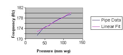
As with the winding system, acoustic coupling is a dynamic process in which the effects vary continuously and rapidly as a pipe organ is played. Modelling it is not as straightforward as in the case of the air supply and various heuristic assumptions have to be made. An organ pipe sometimes emits an audible transient sound (chiff, spit, etc) when it is keyed. However not all do, and that is partly because some organ builders both in the past and today regard them as undesirable. So do many players and listeners. Organ builders can choose either to emphasise or suppress transients if they are good enough at voicing. Transient formation in flue pipes is discussed in detail in [3] which deals with flue pipes, although some of the factors also apply to reeds as well. That article enumerated the main issues which will now be discussed in relation to sound synthesis in digital organs. Aside from the pipe itself, the main factors influencing the attack transient are static wind pressure, fluctuations in wind pressure about the static value, the type of chest, the type of valve and valve opening time. There are also subsidiary factors such as whether conveyances beyond the valve are used to take wind to the pipes. Of these, the only ones which can result in variations in speech from one time to the next (which are the only ones of interest here as explained above) are valve opening time, which translates into keying velocity in a mechanical action, and wind pressure fluctuations. These will now be discussed. The speed at which a note is keyed can influence the attack transient to some extent in organs with a sufficiently responsive mechanical action, though obviously not with pneumatic or electric actions in which the speed at which the pipe valve opens is fixed. The matter was discussed in my paper which appeared in Organists’ Review some years ago, also now available elsewhere on this website [8]. However, even in those cases when the player can modulate transient effects from the keyboard it is doubtful whether many actually do [9]. Nevertheless, by varying those parameters in a physical model which depend on key velocity (which can easily be obtained using standard MIDI techniques) the transient will in turn vary according to keying speed. However this is also possible with sampled sounds. By storing a reasonable number of different attack transients (which only occupy a small amount of memory because they are of such short duration), the appropriate transient for a given key velocity can be automatically selected. It is then a simple matter using standard wave editing techniques to cross-fade the end of the selected transient into the stored steady state waveform. With additive synthesis the matter is not quite so straightforward because it is often difficult to analyse the frequency structure of a transient in enough detail to enable an additive synthesis organ to give a convincing rendering of it. Consequently these difficulties would be magnified if it were necessary to analyse and store a frequency representation, not just of one transient, but of several to correspond with different key velocities. Wind pressure controls the likelihood that a flue pipe will momentarily overblow when it is keyed and thus whether it will emit an attack transient such as chiff, which is when a pipe briefly emits one or more higher harmonics before settling down to stable speech. This is discussed in detail in [3] and only a summary is included here. Figure 3. Measured variation of fundamental frequency with wind pressure for a flue pipe The variation of pitch with pressure for an actual pipe is shown in Figure 3 (blue curve), which demonstrates the well known fact that pipes go sharp if blown harder and vice versa. The pink line shows that the curve can be approximated quite accurately by a straight line except at its ends, which means it is easy to incorporate the frequency versus pressure characteristic in a physical model of a pipe. Eventually an open pipe will suddenly overblow to the octave and a stopped one to the twelfth; this occurred at pressures above 100 mm wg for the pipe represented in the diagram. Therefore if the static wind pressure is set close to this overblowing point it is possible to encourage a pipe to chiff briefly at a higher harmonic before reaching its stable speech regime. Conversely, a lower static pressure will reduce chiff. This is because the brief pressure excursions which often occur at the instant of keying can cause a pipe to overblow and thus emit an attack transient. All these factors are amenable to physical modelling, indeed a proper model must cater for them. However, apart from a few very responsive mechanical actions, opportunities for the player to introduce variations in the type of transient emitted due to wind pressure variations are virtually non-existent. This is simply because a pipe sits on its wind in the manner fixed once and for all by the organ builder, and that is that. Therefore any other form of modelling enjoys little, if any, practical advantage over sampled sounds or additive synthesis in these respects . When a pipe has settled down to stable speech it has reached its so-called sustain or steady state phase. The player cannot influence any aspect of this phase of pipe speech because the key remains depressed to the fullest extent. This is unlike a piano, in which the nature of the sound once the key has bedded depends on the way it was struck in the first place. Nevertheless a pipe does exhibit small variations in its sound during the sustain phase, such as a slight wavering in pitch or “bubbling and burbling”. These can occur for both reed and flue pipes. Even in the unlikely circumstance where there are no wind pressure fluctuations these variations can be triggered because of air turbulence. Turbulence is difficult to model accurately although it can be approached using chaos theory as used in weather forecasting, but it somehow seems unlikely that digital organs would go to the lengths of incorporating chaotic turbulence models. In practice the variations heard will largely be due to wind pressure fluctuations, which can be both random and systematic. Randomness is easy to introduce, whereas modelling systematic fluctuations requires the use of a dynamic wind system model as discussed above. The model should encompass wind pressure effects due to other pipes, either already speaking, coming onto speech or ceasing to speak while the pipe being modelled is in its sustain phase. Acoustic coupling between pipes has been mentioned already, and it also contributes to the small variations which take place during the sustain phase when more than one pipe speaks simultaneously. It is important to understand the ultimate effect of these models, no matter how sophisticated they might be, on the simulated pipes. In the last analysis they can only really affect the pitch and perhaps the amplitudes of each pipe to a small extent. This is because variations in wind pressure will shift the frequency of the fundamental, and thus of the harmonics in the same proportion, as shown in Figure 3. Pitch variations caused by acoustic coupling will also affect the fundamental and all the harmonics in a similar manner. Therefore digital organs using sampled waveforms or additive synthesis can simulate these effects just as adequately as those using physical modelling, provided their synthesis hardware and software is able to render the small but rapid frequency changes which are the outputs of the models. As stated earlier, some commercial sampled sound organs have been doing this for several years. Much of what has been said about attack transients applies to release transients also. However it is probably fair to say that they are less important from a perceptual point of view if only because the detail of release transients is usually submerged within the sound of pipes already sounding plus the ambience of the auditorium. There is also reason to believe that our auditory systems have evolved in a way which makes the onset of a new sound more important to survival of the species than its termination. Therefore we might have more difficulty perceiving the detail of a termination transient than an attack transient simply because of the way our brains are wired. Nevertheless it is useful to review a special case, that of pitch variation as the key is released. To illustrate this, consider the conventional bar and slider chest in which a note is already sounding. The wind pressures in the chest below the pallet and in the groove above it are approximately equal and above atmospheric pressure. The transition to atmospheric pressure occurs chiefly within the pipe itself, at the foot and in any other constricted parts such as the mouth, and maybe at the pallet as well if it is too small for the job. If the key is now released rapidly the pallet will close correspondingly rapidly, leaving the groove still charged with compressed air. Clearly this will dissipate through the pipe more or less rapidly, but the time taken for this to happen is finite. This time interval will depend on several factors such as the wind pressure, the volume of the groove, the number of stops drawn, the types of pipework they represent, etc. But the time involved can be measured and it is typically of the order of tens of milliseconds. What happens to the sound of the pipes during this time?
A
common feature is that the pitch of the pipe will vary before it ceases to
speak. As pipes are sensitive to wind pressure (Figure 3) this is
not surprising. What may be
surprising is the magnitude of the effect.
My measurements suggest that for small flue pipes (such as those of less
than one foot speaking length) the pitch variation can approach a semitone
before the sound ceases altogether. This
is a large variation, and probably the only reason it is not more subjectively
obvious is because of the short period over which it takes place.
Indeed, experiments I have undertaken using electronics for convenience
lead to the conclusion that the pitch change over such a short interval has to
be relatively large for it to have any subjective effect at all.
Thus here we have another example of the transient
phenomena of organ pipes which have some sort of aural effect and, importantly
with a mechanical action, effects which can be controlled by the player in
theory. For if the key were to be
released slowly, the wind pressure in the groove will decay correspondingly
slowly. Thus whatever effects were present in the former case will now be
prolonged. The consequence is that
a physical model must be able to model these effects. However, apart from a few very responsive mechanical
actions, opportunities for the player to introduce variations in the type
of transient emitted are non-existent. Therefore,
as with attack transients, physical modelling probably has little, if any, practical
advantage over sampled sounds or additive synthesis in these respects.
In the latter methods the release transient is incorporated automatically
as a consequence of having captured and/or analysed the sounds of real pipes [11].
Musical instrument synthesis using physical modelling has now been commercially available for about 15 years whereas digital organs using other synthesis methods have been around for about 40. However it is only recently that physical modelling has appeared in digital organs. Physical modelling has without doubt resulted in a step change in the fidelity of simulation of traditional instruments such as the piano, woodwinds, brass and strings. Taking a woodwind instrument as an example, there are many variables characterising the player’s embouchure, the continuously variable blowing pressure and the subtle acoustic mechanism of the tone holes. Also it operates over a frequency range of several octaves. All these variables have been successfully parameterised and incorporated into elaborate and effective physical models. However this is very different to the much simpler case of an organ pipe in which there is no equivalent of the embouchure, the wind pressure only fluctuates slightly about a preset value, there are no tone holes and it only works at a single frequency. This means that the pipe organ is much easier to simulate than orchestral instruments, thus digital organs using conventional sampling and additive synthesis have been able to simulate pipes to a high degree of realism for many years. Capturing the virtually invariant sound of a real organ pipe and embedding it within a digital organ means that it can be re-created to an arbitrary degree of exactness using these conventional methods. It therefore begs the question as to what additional advantages physical modelling can bring to simulating a pipe organ. The answer can only lie in the small variations which occur in pipe speech, small though they are compared to the vast range of expression which any orchestral instrument is capable of. It has been shown in this article that these variations are caused by fluctuations in wind pressure and by acoustic coupling between nearby pipes, therefore they can be simulated by incorporating models for wind pressure and acoustic coupling in any type of digital organ. The corresponding effects on the simulated pipe sounds are limited to small variations in pitch and amplitude, which can both be rendered by modern sampled sound and additive synthesis techniques. Physical modelling can also do these things in principle. Therefore, although it is not disputed that physical modelling is capable of simulating pipe organs to a high degree of fidelity, it seems reasonable to view it as another way to do the job rather than as an intrinsically better one.
1.
“Voicing Electronic Organs”, C E Pykett 2003.
Currently on this website (read). 2.
See http://en.wikipedia.org/wiki/Physical_modelling_synthesis
(accessed on 25 March 2009). 3.
“How the Flue Pipe Speaks”, C E Pykett 2001.
Currently on this website (read). 4.
“How the Reed Pipe Speaks”, C E Pykett 2009.
Currently on this website (read). 5.
“The Tonal Structure of Organ Flutes”, C E Pykett 2003.
Currently on this website (read). 6.
“The Tonal Structure of Organ Principals”, C E Pykett 2006.
Currently on this website (read). 7.
To be rigorous, it is unlikely that key velocity in a digital piano will
be represented to a precision greater than 7 bits because MIDI will usually be
used to convey the information from the keyboard to the computer.
MIDI cannot encode quantities with greater precision than this. 7 bits corresponds to 128 discrete velocity steps, rather
than the continuous variation implied in the text where it is stated that
physical modelling enables any key velocity to be simulated.
However the difference will usually be unimportant in practice. 8.
“Touch Sensitivity and Transient Effects in Mechanical Action
Organs”, C E Pykett, Organists’ Review, November 1996.
Also currently on this website (read). 9.
"The Physical Characteristics of Mechanical Pipe Organ
Actions and how they Affect Musical Performance”, Alan Woolley, PhD thesis,
University of Edinburgh, 2006. 10. It is impossible to model an organ winding system exactly because modelling the air flow in detail would involve the Navier-Stokes aerodynamics equations, and these cannot be solved analytically by any known means. Only approximate numerical solutions can be obtained using powerful computers as used in meteorology and aircraft design. Therefore, like everything else connected with physical modelling synthesis, wind system modelling can only be approximate at best.
11. With sampled sound instruments it is more difficult to merge the end of the sustain phase into the release transient than it is to merge the attack transient into the start of the sustain phase. This is because the length of the sustain phase depends on how long the key is held, which of course is undefined and continuously variable over wide limits. Therefore it might be argued that physical modelling has an advantage here. However this problem was appreciated and solved many years ago in the majority of digital organs once their synthesis hardware and software had become sophisticated enough.
|