


|
|
|
A Second in the life of a Violone
by Colin Pykett
Posted: July 2005 Last revised: 21 December 2009 Copyright © C E Pykett
Abstract There are several articles on this website dealing with how organ pipes speak and the composition of their tones, such as How the Flue Pipe Speaks, The Tonal Structure of Organ Flutes and Voicing Electronic Organs. All can be found on the Complete Articles page, and they all rely largely on the results of my own research into the physics of organ pipes and why they sound as they do. However none of them expose the details which will be discussed in this article, which provides more insight into the processes necessary to achieve a satisfactory understanding of these matters. The article explores the sound of a single Violone pedal string pipe as it comes onto stable speech over a second or so. Personally, I find that such knowledge enhances my admiration for the astonishing beauty of sounds such as these which emerge from nothing more than an enclosed column of air, and I hope that at least some readers will agree.
If you click on the image below you should hear bottom F played on a 16 foot pedal Violone stop, provided your loudspeakers or headphones are good enough (the fundamental frequency is 43.7 Hz).
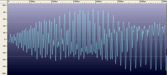
Click on the image to hear a Violone pipe sounding (MP3 file: 174kB) I recorded this example in 1979 at Great Malvern Priory where there is a beautiful four manual organ built by Rushworth and Dreaper in 1927. At the time of the recording the instrument had recently been pronounced so fine by the late Ralph Downes that it should never in future be touched tonally (although that has, unfortunately, happened subsequently). Yet, exactly what is it that you are hearing? In this case, and among other things, you can just hear the church clock chiming (it was late in the evening, and the verger had forgotten I was in the church so he had by then locked me in and gone home. As mobile phones had yet to be invented, I was only able to attract his attention by playing very loudly for a long time). If you have difficulty with the clock, listen carefully as the pipe sound is dying away and you should hear it then. What else? The sound is fine and vigorous of course, as befits a large string toned pipe. It has that rather expensive-sounding purr which is almost exclusively found only in the larger and better quality instruments in this country. Anything else? Can you hear the wind noise due to the turbulence of the air as it emerges from the languid and hits the upper lip of the pipe? The blower in this instrument was also pretty noisy at that time, and there was a lot of escaping wind as well. And what about the way that the pipe comes onto speech? You might have noticed that it takes its time before settling down to stable speech. There is an interval of about a second during which various, continually changing, sounds are emitted. These sounds are called the starting or attack transient of the pipe. The ear and brain assign a perception of curious beauty to this initial phase of speech, which is exactly analogous to the chiffs or other noises which higher-pitched pipes sometimes emit. The leisurely onset of speech of very large pipes is impossible to overcome because it is part and parcel of how they work and it is particularly pronounced for string toned stops, although the detailed structure of the transient can be modified to some extent by a voicer. The leisurely attack is one reason why the higher pitched stops, including mixtures, are so important in a properly designed pedal department. These settle down much quicker, endowing the pedal line with attack and definition to complement the gravitas from the larger pipes. We shall now explore all these matters in more detail (except the clock chimes), and because the attack time of this pipe was about one second, so this article gained its title. The way the sound wave from the pipe evolves in time is shown in Figure 1, which is a snapshot of the first 0.7 seconds of sound after the pallet has opened. This waveform is a depiction of the electrical signal recorded on the tape from a microphone, and it indicates voltage on the vertical axis (positive and negative about a zero line) with time running horizontally. The electrical signal, in turn, is an exact replica of the pressure level of the sound wave in the air experienced by the microphone.
Figure 1. First 700 msec of the waveform
Note how the frequency of the sound reduces considerably as time progresses (in crude terms frequency is indicated by the time between successive zero crossings in the same direction, that is, the gaps between the points at which the waveform crosses the zero line. A short gap means a higher frequency than a longer gap). Thus the sound starts off at a higher frequency than that which is heard once the pipe has settled down to stable speech. It is difficult to draw further conclusions about the frequency structure of the sound merely by examining the waveform however, and to make progress we need to look at a spectrogram instead (Figure 2).
Figure 2. Spectrogram of the first 2 seconds of speech This is a much more complicated picture, so we need to spend some time examining it. It is an attempt to represent three different quantities simultaneously on the two-dimensional page, thus it has a sort of “solid” and 3-d look about it. The three quantities are: Time. This runs away from you horizontally into the distance, according to the scale markings on the right hand side. Unfortunately the markings have become illegible owing to the processes necessary to reproduce the image here, but the time span indicated is about 2 seconds. Frequency. This runs horizontally from right to left, with a range from 20 Hz to 160 Hz. The different frequencies have been assigned the various colours of the rainbow from red (low frequency) to violet (high frequency). Amplitude. Amplitude or strength is measured using the same units (volts) as in Figure 1. It is indicated by the vertical height of the graph above the time-frequency plane. Figure 1 was a plot of voltage against time, whereas here we are plotting voltage against both frequency and time simultaneously. To properly understand the 3-dimensional character of the signal and what it is telling us, it is necessary to look at several pictures similar to Figure 2 but from different perspectives. In effect, you have to imagine you can walk round the diagram and view it from any angle you choose. It is obviously impossible to include all of these views here on account of space, but some important conclusions can be drawn only by examining Figure 2 alone. I included this particular perspective view deliberately because it shows that there are three definite frequencies involved as this Violone pipe comes onto speech. (In reality there are more than three, but to include all of them would mean obscuring the simplicity of the picture). Note that the simultaneous presence of these frequencies cannot be deduced merely by examining the waveform only, as in Figure 1. The three frequencies are the fundamental or first harmonic (coloured yellow), the second harmonic (green) and the third harmonic (blue). The second harmonic is at twice the frequency of the fundamental (i.e. 87.3 Hz), and it sounds the octave. The third harmonic is at three times the fundamental frequency (131 Hz), sounding the twelfth. The simultaneous existence of the several harmonics gives the pipe its characteristic timbre or tone quality, and the way they evolve in time over the first second or so explains why you hear the starting transient of the pipe in the way you do.
Figure 3. The same spectrogram but viewed from a different perspective Although I said earlier it would be impractical to include all the important perspective views of the previous picture, it is useful to look at one more. Figure 3 shows exactly the same data but viewed end on. It is as though you have walked round Figure 2 in a clockwise direction and are now looking at it from the left hand end. This reveals something which could not be deduced easily from Figure 2, that the attack times of the various harmonics are different. The third harmonic (blue) rises quickly to its peak value in about 0.4 seconds before dropping back to a lower level and then bouncing about for a while before stabilising. The second harmonic (green) behaves similarly, though the former perspective of Figure 2 shows that it stabilises rather more quickly. However the fundamental (yellow) takes longer to reach its maximum value but when it does, after one second, it remains stable at that level thereafter. It does not fall back nor bounce around. These behaviours are observable to some extent in the time waveform of Figure 1, where we saw more crudely that the fundamental takes longer to appear and become stable than do the higher frequencies making up the attack transient. With familiarity and experience it is possible to identify additional features in the data. Look at the beginning of the second (green) and third (blue) harmonics in Figure 3. Both rise very quickly to form small subsidiary peaks before their main peaks appear. The alternative view in Figure 2 shows that these initial peaks are actually very slightly lower in frequency as well – it is easiest to spot this for the green curve. In other words, the second and third harmonics begin slightly flat in frequency compared to the frequencies they assume when stable. Figure 2 also reveals that this occurs for the yellow fundamental as well, except that it begins very slightly sharp. Owing to the mathematical limitations of spectrum analysis, these frequency differences cannot be measured precisely but they are less than 2 Hz. Because the various peaks wander around in frequency for a while, it is in fact incorrect to refer to them as harmonics during the attack transient phase because they are not in an arithmetically exact relationship (strictly, harmonics are always exact integer multiples of the fundamental frequency). Therefore it is more correct to call them attack partials during the attack phase of the sound to emphasise this point. At the beginning of the attack transient, the frequencies emitted by the pipe are influenced by its natural frequencies, and these are not exactly harmonically related as explained in [1]. However once the pipe has settled down to stable speech the frequencies it emits are the forced vibration frequencies of the pipe, and these are exact harmonics of the fundamental. During the transient phase, the non-harmonic emissions are pulled progressively into phase-lock with each other as the forced vibration frequencies take control. It should now be obvious that the way a flue pipe comes onto speech is extremely complex. The various partials wander around in frequency and amplitude for about a second in this case before stabilising, an interval which corresponds to roughly 45 cycles of the fundamental. In a general sense this is true for all flue pipes, whose attack transients last for between 10 and 50 cycles depending on several factors, including the type of action, wind pressure, the type of chest and the way they are regulated and voiced. However, narrow scale pipes such as strings (a Violone is a string) take longer to stabilise, whereas flutes are the quickest. When the speech of the pipe has fully stabilised it is said to be speaking in its steady state phase, and because in this phase the frequencies of the partials have become exact integer multiples of the fundamental frequency, we can then correctly refer to the steady state partials as the harmonics of the pipe. What does the frequency spectrum of this pipe look like once it has stabilised in the steady state phase? It is shown in Figure 4, where the fundamental frequency and its harmonics have been identified by the red circles. Unlike the previous diagrams, this one uses a logarithmic (decibel) vertical scale for plotting the amplitude values. This enables a much greater dynamic range to be displayed, in this case a range of 1000 : 1, and the relatively large number of harmonics can be seen clearly (in fact they continue beyond the end of the frequency scale). Near the 7th and 8th peaks are some smaller non-harmonic spectrum lines. These belong to the clock chimes! The grassy nature of the plot between the harmonics is due mainly to blower and wind noise. The characteristic shape of the steady state harmonic spectrum of any flue pipe is largely governed by the closeness of the match between the natural and forced frequencies of the pipe, as explained in [1].
Figure 4. The steady state frequency spectrum of the sound (the harmonics are identified by the red circles) So we now need to explain why these characteristic features of speech occur during the attack transient. However, it is important to mention first that they are not necessarily characteristics of the pipe itself but also of the auditorium in which it is situated. In a resonant building such as Malvern Priory there is a significant reverberation time, which means that sound waves lose little energy when they are reflected from the walls. Consequently they persist for many such reflections before becoming insignificant.
When a pipe in such a building begins to speak, not only does its attack transient take time to stabilise but so also does the structure of the reverberant sound field in the church. While this is happening the various frequencies emitted by the pipe arrive at the microphone or the listener's ears from many directions simultaneously, and this gives rise to the phenomenon of interference. Depending on the relative amplitudes and phases of the direct sound wave from the pipe and all the reflected waves, the measured signal strength of every partial will undergo unpredictable fluctuations until the situation both in the pipe and the building stabilises and the steady state is reached for both. Thus we are dealing here with a situation in which both the sound generator (the pipe) and the environment into which it is radiating (the building) have separate transient responses, the resultant sound being influenced by both in a manner so complex that it is impossible to model or predict it successfully. Moreover, the fluctuations will be different for each and every listening position because the time taken for the direct and reflected waves to arrive at each position will be different.
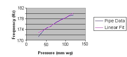
Therefore many details of the spectrograms we have been discussing apply only to the particular position chosen for the microphone when the recording was made. Consequently it is pointless to attempt an explanation of the observed phenomena at an excessively detailed level. (Incidentally, this is a point which seems to be lost on some digital organ manufacturers and other enthusiasts who insist on re-synthesising the sounds of recorded organ pipes to a meaningless degree of detail, especially during the attack transients. Much of the time they are merely re-synthesising the transient response of the building at an arbitrary listening position rather than the sounds of the pipes themselves!). In the case of our Violone pipe the way that the second and third partials apparently bounced around in amplitude during the attack transient was highly likely to have been influenced by the building. However the frequency shifts observed, in which the attack partials start off at slightly different frequencies to those of the steady state harmonics, are purely characteristics of the pipe alone. This is because reverberation, no matter how complex it might be, cannot change the frequencies of the emitted sounds. To continue, then, with the explanation of the observed effects, we should remark that when the pallet opens and wind is admitted to a flue pipe, it may or may not exhibit the sort of complex attack transient that we have observed here. Sometimes there is little or no perceptible transient at all and the pipe reaches its steady state speaking regime over a certain number of cycles without emitting one. This range of behaviours, with or without a transient, can be induced in virtually any pipe by modifying a number of parameters, and it would be quite possible to suppress or modify the transient in the Violone pipe which is the subject of discussion here. Indeed, attack transients have oscillated in and out of favour over the last few centuries as fashions changed. There is some argument over whether Baroque organ builders encouraged or tried to suppress them, but as time moved on there is no doubting the dislike of transients during the Romantic period of organ building of the nineteenth century and into the twentieth. By that time the work of mathematicians such as Fourier and physicists including Rayleigh had led to a greater understanding of acoustics, and this was one reason why new voicing and regulating techniques were invented which enabled transients to be better controlled. Closer to the present day we seem to have rediscovered a liking for audible attack transients in many organs. An important factor governing the transient behaviour of an organ pipe is how close it operates to an overblowing regime. Anyone who has experience of blowing a wind instrument such as a recorder knows that it will fly off to the octave or an even higher note if the player’s breath control and tonguing is inadequate. The painful squawks of aspiring clarinettists, illustrating that the instrument is only too prone to fly to the twelfth of the note played, is another reflection of the same problem. Exactly the same applies to organ pipes, and the voicer can adjust their transient behaviour by exploiting this. Basically, the issue reduces to adjusting the wind pressure at which the pipe speaks, and this is illustrated in Figure 5.
Figure 5. The variation of fundamental frequency with wind pressure for a flue pipe This is a graph of some actual measurements I made on a flue pipe speaking about two octaves higher than the Violone discussed earlier. Thus, although the pitch was different, the general behaviour of the two pipes is similar and common to all flue pipes. The blue curve shows how its fundamental frequency (pitch) in the steady state phase varied slightly with wind pressure. At low pressures the pipe ceased to speak at all, but above this its frequency was accurately linear against wind pressure over a certain range, as shown by the pink line. Beyond a certain critical pressure however, a flue pipe will suddenly start speaking at the octave and the twelfth virtually simultaneously as does our Violone pipe during its attack transient (recall that the octave and the twelfth are the second and third harmonics respectively). This is the case for an open pipe; a stopped pipe overblows to the twelfth only. The overblowing behaviour is not actually shown in the figure, but it began suddenly once the blue curve started to deviate from its straight line character above 100 mm pressure. By adjusting the wind pressure existing just below the languid of a pipe (i.e. at the slit which is called the flue), the voicer can determine where on the curve it speaks. If it sits well inside the straight line region of the curve it will be quite difficult to get it to emit a pronounced attack transient, because we have seen already that the transient consists of an initial burst of the partials associated with overblowing. On the other hand, if it is closer to the top of the curve it will be more likely to overblow as it comes onto speech and thereby emit an attack transient. The wind pressure at the languid of a particular pipe in a rank is adjusted in several ways, for example by inserting wooden plugs into the foot if it is a wood pipe. Or the foothole of a metal pipe can be opened or reduced by working the soft metal. In the case of very large pipes a rotary butterfly valve inserted in the pipe foot is sometimes used. Having heard the pronounced transient of our Violone pipe, it is likely it was speaking pretty close to the point where it would overblow permanently if the wind pressure was increased by a relatively small amount. It should be remembered, however, that wind pressure adjustments as described will also affect the power or loudness of the pipe, and therefore such adjustments are often made to regulate the power across a stop rather than to specifically tailor the transient behaviour of the individual pipes. By virtue of Figure 5, wind pressure adjustments will also affect the tuning slightly, but this can of course be adjusted later by modifying the effective pipe length. Incidentally, this shows how difficult (often impossible) it can be to recover the speech of an old organ that has been altered. Even if the pipes remain in exactly their original condition with all the original foothole plugging etc intact, which is as rare as hens’ teeth, they may have been planted on a different chest with different sized holes in the top board, table and slider. Unless the wind pressures at the languids, not merely at the feet, of all the pipes can be exactly recovered, a restored or reconstructed organ cannot possibly sound as it did originally regardless of the hype foamed about it. Other factors affecting the attack transient include the type of action and the type of chest on which the pipe sits. These govern how quickly the wind pressure rises as the valve opens and in turn they affect any tendency the pipe may have to emit a transient as it comes onto speech.
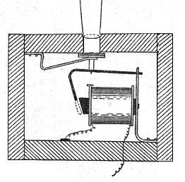
Figure 6. A slider chest A conventional slider chest is shown at Figure 6, and the important point to note here is the groove or channel above the pallet valve and below the pipe feet. This encloses a substantial volume of air which acts as a cushion or buffer when the pallet opens, tending to smooth out the sudden inrush of wind into the pipes. The pallet in such a chest can be operated mechanically, pneumatically or electrically. Of these, only a well designed mechanical action with low or moderate pluck gives the player control over the rate at which the valve opens, thereby also giving him/her control over the way the pipe comes onto speech. Because if the valve opens suddenly the pipe will emit a more pronounced transient than if it opens more slowly. Those who have not experienced this on a mechanical action organ with a moderate amount of pluck have yet to complete their education. It is an important matter, because the ear assigns a high degree of perceptual importance to the rate of onset of a sound and any characteristic transient it might have. Presumably these features have been selected as important to survival as our brains evolved, and subsequently they became equally important to the sounds of music.
Figure 7. A direct electric unit chest By contrast, a direct electric unit chest of the type sketched in Figure 7 has no air cushion between the valve and the pipe. Moreover, because the action is electric in this case, the valve will always open more or less suddenly and its speed of opening cannot be controlled by the player. These factors will combine to produce an air impulse at the languid with a more rapid rise time than that produced by the slider chest, and the pipe will be prone to speak with quite a pronounced chiff or spit unless the voicer takes measures to reduce it. Therefore pipes voiced to speak on one type of chest may speak unsatisfactorily if transferred to another. Sometimes an expansion chamber is provided between the valve and the pipe foot in a unit chest to provide a speaking environment for the pipe more akin to that of the slider chest. Besides adjusting where the pipe operates on the wind pressure curve of Figure 5, the voicer can also reduce the attack transient by cutting grooves or nicks in the languid. These encourage the rapid formation of turbulence in the air flow as it emerges from the languid, and the consequent randomisation of any noticeable transient effects that might otherwise occur. There are several other aspects of the voicer’s art which affect the way a pipe comes onto speech which cannot be covered here. However it is important to note that the various adjustments available to the voicer are all mutually interacting. As an example, he might wish to regulate the power across a rank of pipes by adjusting their footholes, but this will modify their transient behaviour as well. Therefore the selection of a voicing strategy for an organ, such as whether so-called open foot voicing is to be used, depends on what factors in the final sound are thought to be the most important. Leaving the feet of the pipes unobstructed can endow an organ with considerable liveliness and character in some circumstances. This is because the speech of the stops in such an instrument varies markedly from pipe to pipe in terms of their attack transients, but so also does their regulation. This can be adjusted to some extent by varying the width of the flue slit, but it can also lead to a windy and scratchy tone. Therefore unless the pipe scales (the ratio of their diameter to length and the way the ratio varies across the rank) are expertly chosen and match the building, the overall effect of the instrument can be most unfortunate. For example, the trebles may scream or the bass may be over-prominent. The situation can be recovered by regulating the pipework in the conventional manner, but this might involve moving away from the original open foot ideal. Reference 1. "How the Flue Pipe speaks", C E Pykett 2001. Currently on this website (read).
|