


|
|
|
End Corrections, Natural Frequencies, Tone Colour and Physical Modelling of Organ Pipes
Colin Pykett
Posted: 10 June 2013 Last revised: 31 March 2019 Copyright © C E Pykett 2013-2019
Abstract. It is well known that organ pipes have an 'end correction' which makes them sound flatter in pitch than simple theory suggests based on their physical length. Organ builders have developed a good empirical understanding of this effect over many centuries so they can make pipes of the correct length, but a satisfactory theoretical treatment still remains elusive. This is partly because one also has to understand the natural resonant frequencies possessed by an organ pipe - these are quite separate both in theory and practice from the harmonics heard in the sound it emits. Each natural frequency has its own end correction which is different from all the others, and this makes the natural frequencies mutually anharmonic. This differs from the forced harmonics in the sound of the pipe when it speaks because their frequencies are exact integer multiples of the fundamental frequency. Because the interaction between the natural frequencies and the harmonics materially affects the timbre or tone quality of the pipe, it follows that the physical mechanisms of the end correction underlie not merely the tuning of a pipe but its subjective aural effects as well.
This article presents the results of research which demonstrates many aspects of a complex matter. However it largely avoids mathematics, and it also describes a novel experimental technique which reveals the natural frequencies of a pipe. The results are related to the work of other authors, not all of which is confirmed. Particular aspects of accepted wisdom not confirmed by the results here include a nonlinear dependence of end correction on frequency (some previous work suggests it is linear). It is also shown that the natural frequencies are not necessarily "nearly" harmonically related as often assumed.
Results such as these are important to refining the physical models of sound generation in organ pipes which are used in some synthesisers and digital instruments. It is suggested that a reasonable goal for such models would be for them to predict accurately the natural frequency spectrum of a pipe of given dimensions, and this should include such details as the Q-factor of each resonance as well as its frequency and amplitude. It is not clear that all physical models used in digital music have yet reached this level of sophistication.
Contents (click on the subject headings below to access the desired section)
A physical picture of end corrections
The natural frequencies of a pipe
Experimental measurement of natural frequencies
Relation to the physical modelling of organ pipes
Appendix 1 - Derivation of end correction in terms of frequency
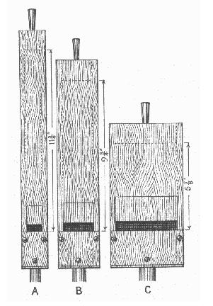
It is well known that an invisible 'end correction' has to be added to the physical length of an organ flue pipe so that it will speak the desired note, and over many centuries organ builders have had to come to terms with this phenomenon. However it is still not a simple matter to predict the end correction accurately for a given pipe using acoustic theory because the correction depends on such factors as whether the pipe is open or stopped at the top, on its scale (the relation of cross-section to length) and on mouth dimensions. That the mouth is a rectangle cut into the side of the pipe is just one factor which makes the acoustic propagation within impossibly difficult to model rigorously, and approximations therefore have to be used. Consequently organ builders continue to rely largely on a venerable body of empirical data which enables them to cut pipes close to the correct lengths, fine tuning then being carried out using stoppers, flaps, slots, slides and the like. This experiential approach persists in the craft today despite many attempts to relate theory to practice, and this is not a criticism. Should there be any doubt, end effects are a significant fraction of the length of the pipe rather than languishing in the background as some trifling academic detail. Their magnitudes were demonstrated by G A Audsley [1] who depicted three pipes in his possession having grossly dissimilar lengths and widths, yet all of them spoke the same pitch. His scale drawing is shown at Figure 1.
Figure 1. Three flue pipes of different lengths and scales which nevertheless speak the same pitch (after Audsley [1])
Thus despite the obvious importance of end corrections in organ building practice, in the sense of knowing how to make pipes of the correct length, the phenomenon in this restricted sense is not discussed in detail in this article. This is because the problems it presents have been solved satisfactorily at a practical level over centuries of trial and error. What concerns us here are the less well known end corrections which apply to the several natural resonant frequencies of a pipe, indeed, the natural frequencies themselves remain commonly misunderstood let alone their end corrections. Following this technical trail will take us into territory allied to the timbre or tone quality of a pipe, and beyond that into the problems of modelling pipe acoustics. 'Physical modelling' is one of today's buzz phrases in digital sound synthesis, so if one cannot model the natural frequencies and their end corrections accurately, then one will not be able to model pipe sounds accurately either. The consequence is that, without such understanding, one will still have to fall back on empiricism and heuristics when developing a satisfactory computer model of how an organ pipe speaks. Physical modelling is of limited value if it cannot model the natural frequencies of a pipe and their individual end corrections, together with other parameters such as the Q-factor of each resonance (described in more detail later).
Many attempts have been made to pull the unruly topic of end corrections under the umbrella of science since the time of Cavaillé-Coll [2], Helmholtz [3] and Rayleigh [4] in the nineteenth century, at both a theoretical and experimental level. However it is fair to say that the literature is characterised more by disagreement and confusion than elucidation, and because of the wide variations which exist one wonders whether some authors were actually talking about something quite different. Thus a definition in their papers would have been valuable, and for this reason end correction as a term used in this article will be defined shortly. At an experimental level, more than one paper describes measurements made using techniques which could not have provided unambiguous or even meaningful results. For instance, a favourite method at one time was to excite a pipe using the fixed frequency from a tuning fork and then vary the length of the tube using water immersion or a sliding stopper until resonances were observed (reference [5] typifies work of this genre). Unfortunately this technique varies two parameters at once - not only the pipe length but its scale as well. In science one must only vary one thing at a time! Since end correction depends on scale as well as on length, which surely must have been known to the authors, their results have to be treated with caution. Matters improved somewhat when the arrival of electronics facilitated the generation of variable audio frequencies, the pipe then remaining of fixed dimensions while the oscillator was adjusted for resonance (see [6] for an example). Even so, this paper concluded lamely that "it is to be hoped that some equation which fits experimental results satisfactorily will soon be found".
Which brings us neatly into the theoretical domain. Since about 1960 the increasing availability of computers probably accounts for the growth of mathematical models (algorithms and equations) to explain end correction phenomena at the expense of experimental work. Yet the results can scarcely be regarded as consistent, either among themselves or with experimental data. As recently as 1999 it was being asserted that the end correction of the natural resonances of a pipe "decreases smoothly with increasing frequency" [7], a result which is not borne out by the experiments to be described here. Theoretical work continues to be done today, partly driven by interest in the digital synthesis of musical instruments using physical modelling. Much of it centres on time-domain methods such as waveguide synthesis [8], but these must reproduce satisfactorily experimental results such as those described later if the model is to be regarded as successful. It is not clear to me whether this has been achieved, as some models at least appear to rely on the vast corpus of practical data which has been painstakingly assembled over hundreds of years by organ builders. Thus such 'models' are merely stuffed full of tables containing end corrections for pipes of given dimensions, or they utilise empirical equations which are forced to fit and thereby regenerate the data. These models will of course work, more or less, and they will also run quickly, which is important in real time digital synthesis. However they do little to enhance a theoretical understanding of the situation.
End correction defined
Before going further it is necessary to define what we mean by end correction. The definition is simple, but it has often been omitted in previous work. In this article the end correction of a pipe is related to the difference in frequency between a pipe of given length were there no end correction, and the actual (lower) frequency of the same pipe when there is an end correction. The definition is cast in terms of frequency rather than length to enable it to be applied to each natural frequency of the pipe as well as to the fundamental (pitch) frequency.
The mathematics is elementary, but to avoid cluttering the main text it has been relegated to Appendix 1. Two equations are derived there for stopped and open pipes, respectively, as follows:
End correction of the nth natural resonance of a stopped pipe = ECn(stopped) = nc/4fn - L (n = 1, 3, 5, ...) equation 1
End correction of the nth natural resonance of an open pipe = ECn(open) = nc/2fn - L (n = 1, 2, 3, ...) equation 2
where:
c is the speed of sound,
fn is the frequency of the nth natural resonance, and
L is the actual length of the pipe.
A physical picture of end corrections
Maybe I have yet to look in the right place, but so far I have not come across a description of how end corrections arise at an intuitive, pictorial level. So I attempt to paint such a picture here of what an end correction actually is. It most certainly is not a simple extension of the constrained air within a pipe sticking up into the atmosphere like an invisible cylinder sitting on top, whose length equals the end correction..
To derive the picture it can be helpful to relate the acoustic radiation occurring from the open top and mouth of an organ pipe to that which occurs from a loudspeaker. So consider first of all a loudspeaker mounted in a baffle or enclosure. When its cone moves it exerts pressure on the air immediately in front of it, the pressure being either a compression or a suction depending on whether the cone is moving outwards or inwards. This disturbance propagates away from the cone into the space in front of the baffle, and while it is still constrained by the baffle at short ranges the wavefront is curved and hemispherical. However, with increasing distance the wavefront (spread over an expanding spherical surface of ever-increasing diameter) becomes large enough to allow it to be regarded as a flat plane rather than curved when it reaches a distant listener. Close to the loudspeaker or an organ pipe the waves propagate in what is called the near field, whereas at larger distances when the wavefront has become plane they are said to be in the far field.
The natural frequencies of a pipe
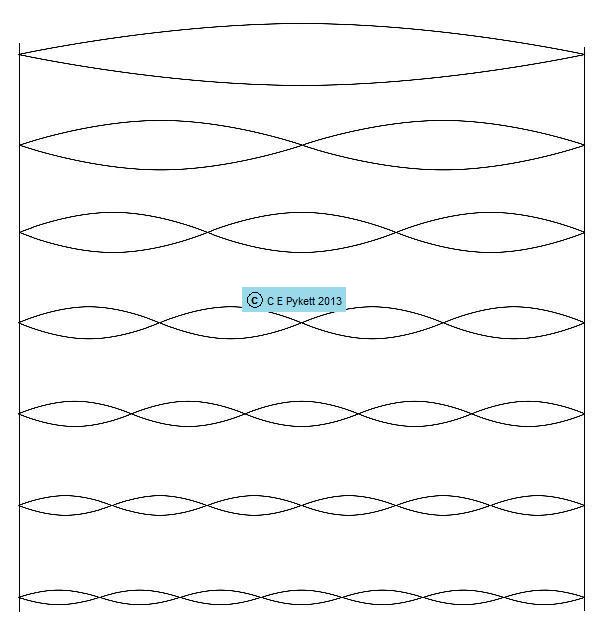
All pipes, and thus flue pipes in the organ, have a retinue of natural frequencies at which they will resonate if excited appropriately. Consider first an open flue pipe. If there were no end corrections either at the top or the mouth (an impossible situation), the fundamental frequency it sounded when blown would have a wavelength equal to twice the pipe length as explained in reference [9]. This would also be the first natural frequency of the pipe. The second natural frequency would have a frequency exactly twice that of the first, and so on. Thus the harmonics of the pipe when sounding would coincide with the natural frequencies. This is illustrated in Figure 2 which shows the standing wave patterns inside the pipe of the natural frequencies and the harmonics. The curves depict the air pressure nodes and antinodes for the first seven natural frequencies. Nodes occur where the vertical width of the pattern is zero, and antinodes occur where the width is a maximum (a useful aide memoire here for those taking science exams is that an antinode - a longer word than node - is wider than a node). At each end of the pipe the pressure of the vibrating wave must be zero (a node) because it is open to the atmosphere at those points and the pressure therefore will dissipate rapidly.
Figure 2. The first seven natural frequencies of an open pipe without any end corrections (illustrated as pressure standing waves along the length of the pipe)
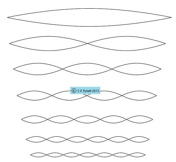
In the real case where end corrections exist at the mouth and top, one possible situation is sketched in Figure 3. Here the end corrections are shown reducing with increasing frequency. It is emphasised that this is only a sketch and not necessarily an accurate depiction of a real situation, but the general trend is correct in that the total end correction (mouth plus top) for the lowest natural frequency is greater than those for the higher ones. This means the standing wave for the lowest frequency is longer than those for the upper frequencies, as shown.
Figure 3. The first seven natural frequencies of an open pipe with mouth and top end corrections which decrease with increasing frequency (illustrated as pressure standing waves along the length of the pipe)
You should therefore be able to see that the upper frequencies are now sharper in pitch than the lower ones, because the standing wave patterns of the latter have in effect been 'stretched' relative to those of the former. In other words the natural frequencies are now mutually anharmonic. Unlike the previous case where end corrections were ignored, the natural frequencies are now quite different to the harmonics in the sound generated by the pipe when it is blown. The harmonics are always exact integer (whole-number) multiples of each other (the second harmonic is exactly twice the frequency of the fundamental, the third harmonic is exactly three times the frequency of the fundamental, and so on). This mismatch between the natural frequencies and the harmonics is an important factor in determining the tone colour or timbre of a real pipe, a subject we shall return to in detail later. The mismatch is entirely due to the existence of end corrections which vary with frequency.
Figures 2 and 3 relate to an open pipe in which all harmonics, both the odd-numbered ones and the even-numbered, are present in the sound when the pipe speaks. In a stopped pipe the situation is different. The top of the pipe is no longer open to the atmosphere but closed by the stopper. This means the pressure must always be maximum (an antinode) at this point rather than zero, otherwise no reflection of the travelling pressure impulses in the air column could take place - if the pressure were zero there would be nothing to reflect back down the pipe. But at the mouth the pressure must be zero as before because it dissipates to the atmosphere. These criteria mean that standing waves having a pressure node at the stopper can no longer exist, and these are the even-numbered harmonics of the pipe. The same criteria also mean that the pipe is now a quarter-wavelength long at the fundamental frequency rather than the half-wavelength of the open pipe, which makes it speak approximately an octave lower than the open one. The effects are illustrated in Figure 4, where the disallowed natural frequencies are marked with the red crosses.
Figure 4. Natural frequencies of a stopped pipe with mouth end corrections which decrease with increasing frequency (illustrated as pressure standing waves along the length of the pipe)
But how can the natural frequencies of a pipe be revealed and how can we measure them if the pipe is not allowed to speak while we are doing so? If it did speak we would only be able to measure its harmonics, which are not the same thing as we have just seen. This conundrum is solved in the next section.
Experimental measurement of natural frequencies
Experiments have been done on various pipes but for the sake of brevity only the results relating to one pipe are included here. This pipe was of wood with internal dimensions 458 by 58 by 46 mm. Its mouth was cut in a wall perpendicular to the larger cross sectional dimension. The pipe was originally stopped and it had been used in an organ to sound the F below middle C (about 175 Hz), but for these experiments its stopper was discarded. The pipe was used both open and closed, but in the latter case it was covered by a wooden lid clamped to the top of the pipe against a compliant sealing gasket. Therefore the physical length of the pipe in both the open and stopped configurations was identical at 458 mm.
The pipe was excited acoustically by a small loudspeaker mounted externally above its mouth. This was a 'postage stamp' speaker taken from a computer monitor, and it could scarcely be described as anything remotely approaching high fidelity. However for the purposes of these experiments this did not matter because it was calibrated to enable its response to be accounted for when analysing the results. The speaker was supplied with computer-generated white noise, and the sound at the far end of the pipe was picked up by an electret capacitor microphone with a substantially flat frequency response. A spectrum analysis was performed on the microphone signal, 35 successive spectra being averaged to reduce the statistical fluctuations inseparable from the use of white noise. This acoustic analysis technique embodies some novel aspects and it is described in more detail elsewhere on this website [10].
Stopped pipe
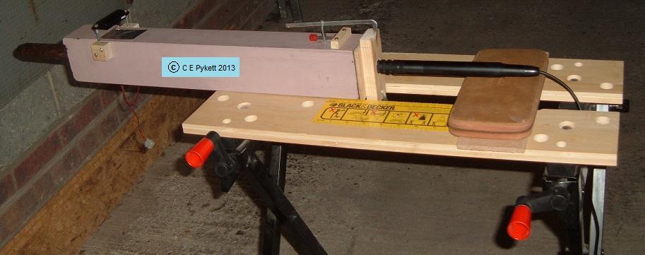
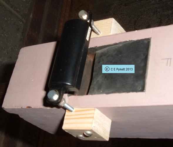
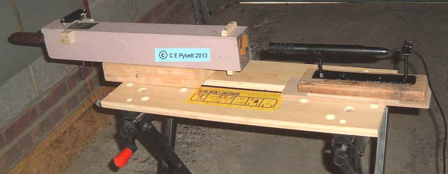
The general experimental set-up for making measurements on a stopped pipe is shown in Figure 5 and a closer shot of the loudspeaker is in Figure 6.
Figure 5. Stopped pipe set-up for measuring natural frequencies - general arrangement
Figure 6.
Stopped pipe set-up for measuring natural
frequencies - loudspeaker mounted at pipe mouth
The speaker was mounted on long bolts so that its distance from the mouth could be adjusted until its presence was not disturbing the acoustic behaviour inside the pipe appreciably. This was judged when further increases in distance resulted in undetectable changes to the natural frequency spectrum. The microphone was mounted at the closed end of the pipe in a tight-fitting wood flange to reduce reception of the direct sound from the loudspeaker tracking along the outside of the pipe. It listened to the sound within the pipe through a 3 mm hole bored in the end cap.
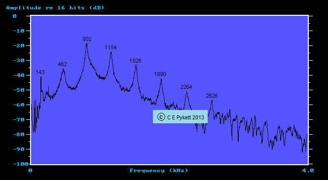
The natural resonances of the pipe are revealed clearly in Figure 7, and their frequency values are shown. Remember that this is not a frequency spectrum of the pipe when blown with wind - the peaks do not represent the harmonics of its sound when speaking. They are the natural resonant frequencies of its air column while the pipe as a sound generator is silent. The pipe is amplifying the frequencies present in the white noise signal from the loudspeaker at which it resonates naturally.
Figure 7. Measured natural frequency spectrum of a stopped pipe (uncorrected for loudspeaker response)
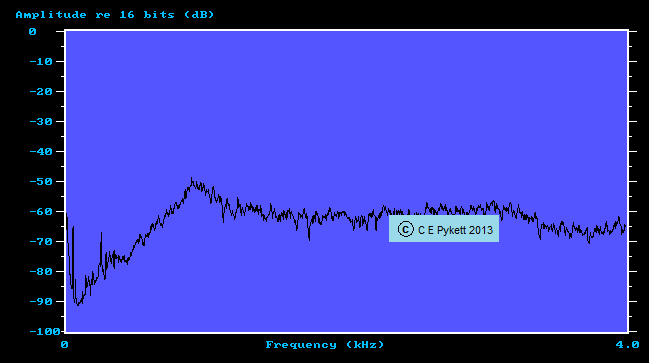
However this plot is not corrected for the loudspeaker frequency response, which is shown in Figure 8 (it was measured as described in reference [10]). The two very sharp low frequency peaks here were due to ambient noise and low level power line pickup at 50 Hz and they can be ignored. Above these the spectrum level rises to reach a peak at about 900 Hz before falling away again. This, together with the general lack of bass, gave rise to a most unpleasant 'tinny' sound when this speaker was used in the computer it was originally pulled from. Obviously, this response had to be subtracted from any measurements made using this item before the results would be useable..
Figure 8. Measured frequency response of the loudspeaker used to excite the pipe resonances
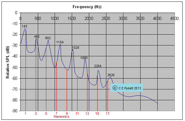
The natural frequency spectrum, corrected for the loudspeaker response and then smoothed, is at Figure 9 (blue curve).
Figure 9. Measured natural frequency spectrum of a stopped pipe (corrected for loudspeaker response)
The significance of the red lines will be discussed later, together with the corresponding data for an open pipe. Measurements on the latter will now be described.
Open pipe
The slightly different experimental set-up for the open pipe is shown in Figure 10. It was generally similar to that for the stopped pipe except that no cap was used, and the microphone was placed on a horizontal stand close to the open end of the pipe. As with the loudspeaker, its separation from the pipe was increased until no further effect on the resonance spectrum was detectable.
Figure 10. Open pipe set-up for measuring natural frequencies - general arrangement
The natural frequency spectrum obtained, corrected for the loudspeaker response and smoothed as before, is at Figure 11.
Figure 11. Measured natural frequency spectrum of an open pipe (corrected for loudspeaker response)
It is of interest that the peak to valley ratios of the larger peaks are comparable with those for the stopped pipe in Figure 9. This suggests that direct leakage of sound from loudspeaker to microphone was unimportant because significant leakage would have otherwise elevated the valleys by raising the noise floor of the whole graph. Thus, even though the microphone in this case could not be shielded as easily from the direct sound, it seems to have been a minor issue. It is also worth mentioning that although neither set of measurements was derived in anechoic conditions, reflections from nearby boundaries did not seem to have affected the results significantly, at least over the limited frequency range of 4 kHz which was analysed. This conclusion was reached because such reflections are invariably obvious to the eye in frequency plots of the sort presented here. They manifest themselves either as pronounced scatter or periodic ripples in frequency on the graphs, or both. Examples of such phenomena are shown and discussed in detail elsewhere on this website when the response of a loudspeaker in a room was under investigation [10]. Therefore, as they could not be detected visually, it is reasonable to assume they were of little account in this case.
These results for the open and stopped pipes will now be discussed in more detail.
Both the stopped and open pipes had a well-defined retinue of 7 or 8 natural frequencies extending to about 2500 Hz in round figures, as shown by the blue curves in Figures 9 and 11 respectively. The relative amplitudes in decibels of the resonances decreased approximately linearly against frequency in both cases, but those for the stopped pipe fell away much more quickly than those for the open one. For the stopped pipe they decreased by about 43 dB and for the open one by about 13 dB, in both cases over a similar frequency range (2500 Hz approximately). This result is of significance and it will be discussed later in connection with the timbre or tone quality of the pipe when it spoke in the two configurations.
Both sets of natural frequencies were significantly anharmonic, as expected. The frequency of each resonance is noted on the two graphs, and it can be verified easily that the frequency values are not integer multiples of the lowest frequency in either case. This would have been so if they were harmonically related. In fact the upper frequencies are significantly sharp compared to what they would have been had they been harmonically related to the lowest, a feature which was explained earlier and shown to be entirely due to end corrections which reduce with increasing frequency (see the section entitled the natural frequencies of a pipe above).
Another way to detect anharmonicity in the data is to examine the frequency differences between successive pairs of resonances. If the natural resonant frequencies were harmonically related, each difference would be the same. However the difference values in Table 1 show that this was not the case.
Table 1. Frequency differences between successive pairs of natural frequencies (Hz)
The two mean values deviate less than 9% from the theoretical speaking frequency of an open pipe of this length (458mm) with no end correction, which would be 375 Hz. However the first difference in each data set is significantly smaller than all others in the corresponding sequences. If these values are discounted, the mean values become 361 Hz (stopped) and 350 Hz (open), bringing them even closer to 375 Hz. This suggests that some phenomenon is at work which affects the lowest frequency or frequencies more than the higher ones, and that it will be instructive to examine the end correction of each natural frequency. This is done below.
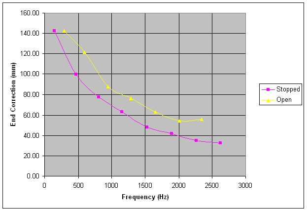
End correction versus frequency The end correction for both stopped and open pipes was defined in equations 1 and 2 above. These were applied to each value of natural frequency so that its end correction could be calculated. Plotted against natural frequency, the results are shown in Figure 12.
Figure 12. Variation of end correction versus natural frequency for the stopped and open pipes
It is obvious from these curves that the lowest two or three natural frequencies have much greater end corrections than the higher ones. In fact the lowest natural frequencies of both the stopped and open pipes have the same value of end correction, which is some 31% of the physical length of the pipe. As remarked earlier, this confirms the significant magnitude of end corrections even for ordinary organ pipes of unexceptional scale such as the one used here.
The results in this graph do not confirm theoretical work elsewhere suggesting that the end correction tends to zero in the high frequency limit [7]. Although the end correction does reduce with increasing frequency, there is little visual evidence that the asymptote will eventually reach zero. Moreover, the theoretical prediction that the end correction of the natural resonances of a pipe "decreases smoothly with increasing frequency" [7] is certainly not confirmed by the nonlinear variations seen in Figure 12. These are examples of where acoustic theory clearly has some way to go before it tallies with reality.
The measured end correction of a stopped pipe can only arise at the mouth whereas that for an open one arises at both the mouth and the top. It is often said that the mouth correction exceeds that at the top, sometimes by a factor as large as five or more. It is unclear to me whether this belief stems from actual measurements or from theory alone, and since certain theoretical and experimental work leaves something to be desired as we have noted already, it seems appropriate to investigate the matter further.
Consider the curve of end correction against frequency for the open pipe (the yellow curve in Figure 12). Each point on this curve presumably represents the total end correction made up from contributions at the mouth and the top. Therefore by subtracting the mouth correction obtained from the stopped pipe (pink) curve at a given frequency, we might expect to arrive at the correction due to the open top only. The data show that the mouth plus top correction of the open pipe at its first natural frequency (286 Hz) is 143 mm. That for the mouth of the stopped pipe at this frequency is about 122 mm, thus the difference between them - 21 mm - is usually taken to represent the top correction only. This is indeed far less than that at the mouth. Similarly, it can be verified easily that all the other natural frequencies of the open pipe have end corrections at the top which are smaller than those at the mouth, though the differences between them reduce with increasing frequency.
A questionable aspect is that the analysis above, based on accepted wisdom, assumed that the total end correction of an open pipe was the simple sum of those at the mouth and the top. Moreover it was then assumed that when the pipe was covered, the mouth correction at a given frequency will remain the same as when it was open. These assumptions are those used everywhere else in the literature. However there is in fact little justification for them, and one can be excused for taking them with a pinch of salt. In fact, one should so take them.
The influence of end corrections and natural resonances on tone quality It has been established for well over a century (at least since the time of Helmholtz [3] if not before) that the subjective tone quality or timbre of a pipe when it speaks is influenced strongly by the relative proportions of the harmonics in the sound. Note that the harmonics are not the same as the natural frequencies of the pipe we have been considering so far. The harmonics exist at frequencies which are always exact integer (whole-number) multiples of the fundamental frequency or first harmonic, whereas it has been demonstrated above that this does not apply to the anharmonic natural frequencies of the pipe. Because the pipe resonates at each natural frequency, it is capable of amplifying by resonance a particular harmonic if the latter has a frequency near to that of a natural frequency. Consequently the natural frequencies modify the acoustic spectrum of the sound generated at the mouth of the pipe, much as a filter in electronics affects the harmonic structure of a previously-generated audio signal passing through it. Therefore the natural frequencies of a pipe exert a profound effect on the tone quality of the pipe when it speaks.
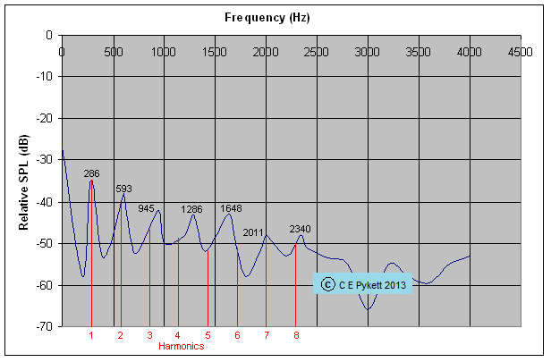
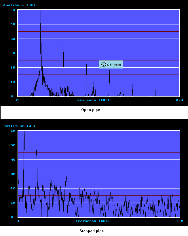
To quantify the matter further, the harmonics generated by the pipe used for the experiments here are plotted as the red lines on the natural frequency spectra in Figures 9 and 11. Their positions along the frequency axis are determined solely by the frequency of the fundamental or first harmonic, because all the other harmonics will then lie at integer multiples of the fundamental. The fundamental frequencies of the pipe used here were measured by blowing it when it was both stopped and open, and then applying a high resolution spectrum analysis to its sound in the two cases. When blowing the stopped pipe the 3 mm hole in its end cap was closed off - this was used previously to allow the microphone to pick up the natural frequencies. The two frequency spectra are shown in Figure 13 (NB note that the two plots have different frequency scales)..
Figure 13. Frequency spectra of the open and stopped pipe when blown (NB: heed the different frequency scales)
Several points are of interest. The fundamental frequency of the open pipe when speaking was 286 Hz which coincides exactly with that of its first natural frequency. The fundamental of the stopped pipe was at 150 Hz, slightly sharp of its first natural frequency which lay at 143 Hz. This was because the 3 mm hole in its cap was open to the microphone when recording the natural frequencies but closed when the pipe was blown. There was an audible difference of about a semitone between the pitch of the pipe blown with the hole open compared to its pitch when the hole was closed. This corresponds to the frequency difference observed here, where the two values (150 and 143 Hz) differ by about 83 cents or again nearly a semitone. When making the previous measurements with the hole open to the microphone the effective length of the pipe changed somewhat, resulting in a slight shift of the first natural frequency of the air column. Therefore it is confirmed that the speaking frequency of both the open and stopped pipes was effectively that of the first natural frequency in both cases within the limits of experimental error, as other work has suggested. (See also note [11]).
Other than the fundamental frequencies, Figure 9 and Figure 11 show that there is little systematic correspondence between the higher natural frequencies (blue curves) and the harmonics of the pipe when it spoke (red lines). The closeness of a particular harmonic to a natural frequency peak determines how strongly that harmonic will be amplified by the pipe. This does not mean that a harmonic will not be heard at all if it does not coincide with a peak, but merely that it will not be so strong in the emitted sound. The sharpness of a peak also plays a role here in that it would be necessary for a harmonic to be close to the peak frequency when the peak is sharp if it is to be amplified, whereas if the peak is broader then the harmonic might still receive appreciable amplification when it is further away. Peak sharpness is defined by the Q-factor of the resonance, defined as the ratio of the peak frequency to its width when its amplitude has fallen by 3 dB. Therefore the Q-factors of the natural frequencies of a pipe also play a role in determining its timbre as well as their frequencies. The Q-factors can be estimated from the results of the experiments described here. Suffice it to say that some theoretical predictions related to Q-factor fall well outside the results obtained in these experiments on a real pipe.
However there is also another important factor governing the amount by which a harmonic might be amplified by a pipe resonance. It was noted earlier that the relative amplitudes in decibels of the natural frequencies decreased approximately linearly against frequency in both cases, however those for the stopped pipe fell away much more quickly than those for the open one. For the stopped pipe the amplitudes decreased by about 43 dB and for the open one by about 13 dB, in both cases over a similar frequency range (2500 Hz approximately). This is a significant difference, and it means that the open pipe will not attenuate the harmonics as much as the stopped pipe would, regardless of how near a harmonic might lie to a natural resonance peak. This is reflected in the spectra of how the stopped and open pipes actually spoke in Figure 13, which show that the open pipe had more harmonics in its spectrum than the stopped pipe. It also explains why there is more 'grass' in the stopped pipe spectrum - this corresponded to the subjective sound of the pipe which was noticeably noisier and breathier than when it spoke in the open configuration. The stopped pipe was also subjectively much quieter than the open one. Yet another factor is that an open pipe emits energy from two apertures whereas a stopped one emits the sound from only one. Still another concerns the number of harmonics - an open pipe radiates both the odd and even harmonics whereas a stopped one the odd ones only. Since the acoustic power of a pipe is contained in its harmonics, fewer harmonics will result in less power provided other aspects remain comparable. All these factors suggest that the stopped pipe was a much less efficient converter of the energy in the input air stream into acoustic energy than was the open pipe.
Notwithstanding the above discussion, the harmonic structure of a pipe when speaking is not solely influenced by the way its harmonics interact with its natural resonances, important though this is. The harmonic structure of the waveform generated at the mouth in the first place also plays a part. One important aspect concerns the amount by which the upper lip is offset from the air jet issuing from the flue slit. If the lip sits exactly above the flue, as it often does in a wooden pipe, the air jet considered as a pulse generator will oscillate into and out of the pipe with a more or less symmetrical mark space ratio of about 1 : 1. This is similar to the square wave used in electronics which contains only the odd harmonics. But if there is an offset between lip and flue, or if the voicer directs the jet slightly away from the lip by adjusting the languid, then the pipe is driven instead by an asymmetrical pulse waveform which will generate both odd and even harmonics. This is a somewhat simplified picture of the harmonic generation mechanism, and in a real pipe the even harmonics are never completely absent. Nevertheless, harmonic generation at the mouth has to be considered as well as the interaction between those harmonics and the natural frequencies of the pipe itself if the spectrum of the emitted sound is to be properly understood.
To summarise at the simplest level, a flue pipe speaks with a fundamental very close to its first natural frequency. The higher order natural frequencies then act as an asymmetrical comb filter which modifies the harmonic spectrum generated by the interaction of the oscillating air jet with the mouth. The comb filter is asymmetrical because its 'teeth' are not equi-spaced in frequency. The asymmetry arises because of the variation of end correction with frequency.
Relation to the physical modelling of organ pipes
Some synthesisers and digital instruments use physical models of organ pipes in the form of algorithms and equations to synthesise their sounds, as an alternative to using sound sampling or additive synthesis [8]. It should be clear from the foregoing that a physical model must be able to reproduce convincingly the natural frequency spectrum of a pipe of given dimensions if the model is to be regarded as successful. The model should predict such details as the Q-factor of each resonance as well as its frequency and amplitude. In turn this means the model must also be able to predict the variation of end correction with frequency. It is unclear whether all models have this capability. At least some seem to devote considerable attention to the minutiae of air jet formation and oscillation (no problem there of course) but this is sometimes at the expense of modelling the air column of the resonating tube. In some cases the latter is only modelled rather crudely as the simplest form of acoustic waveguide, and then it is difficult to see how the end corrections as a function of frequency can be derived. In turn this implies that the natural frequency model will be similarly deficient, together with the way the natural frequencies affect the tone colour of the pipe.
The work described here has shown that the subject of end corrections is complex and many-facetted. Historically it has caused confusion for well over a century and a satisfactory description of the phenomena continues to elude theoreticians. It is my experience that the subtleties of organ pipe sounds at the level of detail examined here still lie somewhat beyond the grasp of physics, and therefore it can be argued that the best way to capture and resynthesise their sounds is simply to record them. This implies that, despite its shortcomings, sampled sound synthesis might still remain the best technique for synthesising organ pipe sounds.
How can the actual sounds of real pipes when rendered by a good sound sampler be considered inferior to modelling them mathematically as some claim? Such a notion must surely rank as perverse?
This article has described experiments which reveal the natural frequencies of a stopped and open pipe using a technique with some novel features. The results of other authors were confirmed in that these resonances were shown to be anharmonic owing to the frequency dependence of their respective end corrections. It was also shown how the interaction between the natural frequencies and the harmonics generated when the pipe speaks materially affects the tone quality of the pipe.
The somewhat confused state of knowledge of end corrections and related phenomena at both a theoretical and experimental level was remarked on. Particular aspects of accepted wisdom not confirmed by the results here include a highly nonlinear dependence of end correction on frequency (some previous work suggests it is linear). It was also shown that the natural frequencies are not necessarily "nearly" harmonically related as often assumed.
It was suggested that a reasonable goal for a theoretical model of sound production in organ pipes would be for it to predict accurately the natural frequency spectrum of a pipe of given dimensions, and this should include such details as the Q-factor of each resonance as well as its frequency and amplitude. It is not clear that all physical models used in digital music have yet reached this level of sophistication.
1. “The Art of Organ–Building”, G A Audsley, New York, 1905
2. "De la Détermination des Dimensions des Tuyaux par rapport à leur Intonation", A Cavaillé-Coll, Académie des Sciences, Paris, 23 January 1860
3. “On the Sensations of Tone”, an English translation by Ellis in 1872 of the German original by H L F von Helmholtz, Brunswick, 1865
4. Lord Rayleigh, Philosophical Transactions, (161), 1871
5. "Effect of Frequency on the End Correction of Pipes", S H Anderson and F C Ostensen, Physical Review (31), February 1928, p. 267
6. "End Corrections of Organ Pipes", A T Jones, Journal of the Acoustical Society of America (12), January 1941, p. 387
7. "The Physics of Musical Instruments", N H Fletcher & T D Rossing, New York, 1999
8. "Physical Modelling in Digital Organs", an article on this website, C E Pykett, 2009
9. "How the Flue Pipe Speaks", an article on this website, C E Pykett, 2001
10. "Equalising Loudspeaker Sensitivities", an article on this website, C E Pykett, 2009
11. A further potential source of discrepancy between the first natural frequency and the fundamental frequency of the pipe when blown is the slight variation in pitch which occurs with blowing pressure in any organ flue pipe. This was measured for the pipe used here and found to be ± 1.4% about its mean frequency over the range of pressures for which the pipe would speak (see Figure 7 in [9] for a curve illustrating the variation in pitch with pressure for this pipe). However this is a much smaller deviation than that mentioned in the main text (first natural frequency = 143 Hz; first harmonic = 150 Hz; a discrepancy of nearly 5%). Therefore the variation of pitch with blowing pressure can probably be discounted as a source of major error in this work.
12. "The acoustic radiation field of organ pipes", an article on this website, C E Pykett, 2017
Appendix 1 - Derivation of end correction in terms of frequency
Let the physical length of a pipe be denoted by L, measured internally from its languid to the top (or the underside of its stopper if closed). The wavelength of the fundamental frequency emitted by the pipe if there were no end correction would then be 2L if the pipe is open, and 4L if the pipe is stopped. This is because an open pipe with no end correction would be half a wavelength long, and a stopped pipe with no end correction would measure one quarter of a wavelength. These assertions are justified in detail in another article on this website [9].
The relation between frequency and wavelength involves the speed of sound: sound speed equals frequency multiplied by wavelength. Thus the fundamental (pitch) frequency or first harmonic of the open pipe would be c/2L and that of the stopped pipe would be c/4L where c is sound speed.
In practice there is an end correction for both types of pipe. For the open pipe a correction exists at the top and at the mouth, whereas for the stopped pipe it exists at the mouth only. In both cases the end correction(s) make the pipe seem longer than it actually is.
For an open pipe let the first natural resonance have a frequency f1. The corresponding wavelength is thus c/f1 , and the effective length of the pipe is c/2f1 because the pipe is half a wavelength long for the first resonance. The second resonance at frequency f2 has a wavelength c/f2 . But in this case the effective length is also equal to c/f2 because now the pipe is a whole wavelength long for the second resonance (see the diagram illustrating the standing wave patterns in Figure 3 above). Proceeding similarly for the other resonances, it can be shown that the effective length of an open pipe for the nth natural frequency is given by Leff(open) where
Leff(open) = nc/2fn
fn is the frequency of the nth natural resonance (n = 1, 2, 3, ...). Therefore the end correction for the nth natural resonance is given by
ECn(open) = Leff(open) - L = nc/2fn - L (n = 1, 2, 3, ...)
For a stopped pipe there are two differences to take into account. One is that the effective length of the pipe is now a quarter-wavelength at its fundamental frequency, not a half-wavelength. The other is that only the odd-numbered resonances can exist for a stopped pipe (see Figure 4 above). Thus similar reasoning to that just given but applied to a stopped pipe gives an end correction for its nth natural resonance as
ECn(stopped) = nc/4fn - L (n = 1, 3, 5, ...)
|