


|
|
|
Creating Sample Sets for Digital Organs from Sparse Data
Colin Pykett
Posted: 24 February 2013 Last revised: 9 July 2014 Copyright © C E Pykett 2013 - 2014
Abstract. This article considers the problem of generating a complete sample set for a digital sound sampler, comprising an independent and different sample for each note, from sparse or incomplete data. The common technique of stretching a sample across a range of notes (keygroup) was not used because this results in an identical timbre or tone quality for each note of the keygroup. Moreover, that timbre then changes abruptly from one keygroup to the next. These deficiencies sound artificial and unsatisfactory. Instead, the approach here uses all raw samples directly in the sampler, and in addition reference spectra are also derived from them. Interpolation from the reference spectra is then performed to create a unique harmonic spectrum for each of the 'missing' samples, which are then generated using additive synthesis. The problem of restoring the necessary realism to the synthesised sounds is illustrated by describing in detail how an attack transient can be analysed and then incorporated in a sample as it is synthesised.
The article emphasises the need for special purpose software tools, not only to implement some stages of a rather complex process in the first place, but to realise them in a time-efficient manner. These tools are deliberately written as stripped-down command line applications which are suitable for batch-processing the hundreds or thousands of samples needed for a high quality digital organ. Examples of the operations carried out include automatic harmonic identification, interpolation, additive synthesis, calculation of loop points and some aspects of transient generation.
These techniques enable a complete sample set to be built from a sparse one using features of both sampling and additive synthesis - the real samples can be used directly in a sound sampler, and they are also analysed to enable the remaining samples to be generated by interpolation followed by additive synthesis. This arguably makes the best of both worlds. Thus all samples in the complete set are based directly on real pipe sounds, which they would not be if they were derived using an approach such as physical modelling.
The widely-available sparse sample set of the Stiehr-Mockers organ at Romanswiller in France by Joseph Basquin is used to illustrate the points made in the article. The 265 original samples in this set were expanded to 923, of which 133 had attack transients.
Contents (click on the headings below to access the desired section)
Dealing with sparse sample sets
Step 1 - spectrum analysis and Automatic Harmonic Identification (AHI)
Step 2 - derive interpolated spectra across each keygroup
Step 3 - generate the intermediate samples
The Expanded Romanswiller Digital Organ
This article addresses the creation of sample sets which define organ pipe sounds for digital organs or virtual pipe organs of the sound-sampler variety. However it is not a general treatise covering the topic from first principles because that would require a complete book rather than just a web page. Rather, it concentrates on the particular problem of how to generate a complete sample set from sparse data in which relatively few raw samples are available. This is a problem I have faced many times when trying to re-create the sounds of organs which no longer exist in their original form, and in these cases it is obviously impossible to develop an authentic sample set simply by recording the sound of each pipe as is usually done by sample set producers. Even with this restricted scope the article cannot cover every nuance of the topic, but I have posted it because of the number of enquiries received about the methods used to develop the various simulations described elsewhere on this site [1]. But in other ways the article is not fully comprehensive either. For instance, if no samples are available at all, then obviously one has to invoke a broader repertoire of techniques than those described here. But hopefully the article will give a flavour of one approach to the problem out of the several which are possible when a complete set of samples is not available.
My simulation system which renders the samples is called Prog Organ, though the techniques described are applicable directly to the preparation of samples for any sampler-based musical instrument simulator. They also have some relevance to organs or synthesisers using additive synthesis or (less directly) physical modelling. However a point which needs to be emphasised at the outset is that, in my experience, some special tools are required in order to implement the techniques. This is because standard waveform processing packages do not offer a sufficiently wide range of capabilities for the specialised requirement discussed here, therefore it was necessary to write some custom software to implement certain functions. One pressing reason for this was the need to automate a potentially very tedious and long-winded procedure as far as possible, bearing in mind that whatever methods are adopted for generating each sample, they have to be multiplied hundreds or thousands of times to produce the complete sample set. Therefore automation and efficiency issues are paramount. These aspects are discussed in more detail later on.
The techniques outlined in the article are illustrated using the sample set recorded on the Stiehr-Mockers organ at Romanswiller, Alsace in France [2]. This is because currently it is free and widely used. The situation might have changed since, but the version of this sample set which I obtained some years ago was 'sparse' in the sense used here in that no more than three sound samples per octave (one every four notes) were available for most stops, and some had fewer. Therefore this version forms a good vehicle on which to base the discussion.
This article is one of several on the site covering various aspects of voicing digital organs [3], and you might like to refer to them if you desire additional background information.
Dealing with sparse sample sets
An obvious and widely-used approach when there is an incomplete set of waveform samples for a particular stop is to duplicate or 'stretch' each one over a range of notes (consecutive semitones), often called a keygroup. Some commercial sample editors allow this to be done easily and rapidly using their on-screen graphical user interface, the pitch of each note in the group being adjusted automatically at the same time. In fact it is the ease of doing it which has probably encouraged the practice. For some other products a more painstaking series of operations is required in which each duplicate (identical) sample has to be imported several times into the sampler, associated with the correct note, and its pitch then adjusted manually. However in both cases the end result is the same - the timbre or tone quality of each note in the keygroup in terms of its harmonic structure is identical. This alone is artificial and unsatisfactory. But worse, that single timbre often changes abruptly from one keygroup to the next, and of course the ear can detect this easily. Other undesirable artefacts include identical attack and decay transients and wind noise across the group, but coupled with a completely artificial change of pitch of these artefacts from one note to the next. Such shortcomings also offend the ear. Attack transients and the like simply do not sound like this in a pipe organ!
The approach described here differs in that the harmonic structure of each note in the range between two raw samples is varied gradually rather than remaining identically the same. Therefore each note in the keygroup sounds slightly different, just as adjacent notes do on a real organ. In some cases the differences are virtually imperceptible, in others they are more obvious. This behaviour also mirrors the pipe organ. Using these techniques there is never a sudden jump in timbre between one keygroup and the next as there can be when using sample-stretching. These desirable attributes occur because each intermediate note has a harmonic spectrum which has been interpolated mathematically, harmonic by harmonic, using the frequency spectra of the two raw samples which bracket the keygroup and act as reference points for it. Moreover, if a particular raw sample possesses distinct characteristics such as an attack transient, that characteristic is not slavishly coped and applied to every other interpolated note in the keygroup as it would be if using sample-stretching. The transient is only applied judiciously and selectively to certain notes, just as it would arise across a real rank of organ pipes. A method for extracting the salient features of attack transients and then 'attaching' them to certain of the derived, interpolated, notes is also described.
In what follows, the raw samples which bracket each keygroup are referred to as 'voicing points' because they define the (interpolated) voicing characteristics of that group. In this connection it should be noted that it might not always be possible to use each raw sample directly in the finished sample set even though they can all be used as voicing points. This paradox arises because some samples might be of such poor quality that they cannot be used directly as waveforms in the rendering engine. Examples of problems which can occur include excessively low signal to noise ratio, action noise which cannot be removed without degrading the sample to an unacceptable extent, interfering noises such as clock chimes, difficulty in generating undetectable loop points, etc. However in most of these difficult cases, sufficient information can nevertheless be extracted from the sample to enable synthetic samples to be generated which can still serve as voicing points. The methods used to achieve this are similar to those employed in synthesising the interpolated notes between the voicing points, and these methods will now be described.
In summary, the following processing steps are performed:
These steps are now discussed in detail.
Step 1 - spectrum analysis and Automatic Harmonic Identification (AHI)
Spectrum analysis is easy and routine today and virtually all waveform processing applications offer it, even the free ones. However, when the spectrum gets thrown up on the screen I used to ask myself "so what?". Being able to see a plethora of harmonics is all fine and dandy, but what does one do with them thereafter? This question assumes serious proportions when there are many harmonics, because manually reading off their amplitudes and copying the numbers into (say) a spreadsheet is not only impossibly tedious, but error-prone as well. Therefore I developed the following method for rapidly identifying the harmonics and saving the amplitude of each one. This is an example of the automated signal processing I referred to earlier, as well as demonstrating the need for special purpose software tools designed for this application.
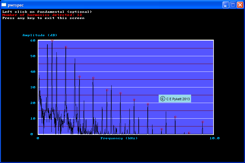
Figure 1 shows the harmonic spectrum of bottom C of the 8 foot Trompette stop on the Grand Orgue of the Romanswiller organ. In this picture 62 harmonics are visible. We know this because the computer tells us so in the top left corner - we do not need to count them. But how did it know? The answer lies in the little red circles which sit on top of each harmonic. They illustrate the output of my AHI algorithm (Automatic Harmonic Identification), and they appear instantaneously if you click with mouse somewhere near the fundamental frequency. They allow you to confirm visually that the algorithm did indeed find the harmonics in a sensible manner (occasionally it does not and then you have to try again). But the more important aspect of the program is that the computer has also found all the harmonic amplitudes, and it will write them to a file if you so desire. Normally you do so desire, and if the file is of type CSV (comma-separated variables), this can then be read by lots of other applications. Therefore you can transfer this important data set, a complete and accurate version of the spectrum in numbers, into an Excel spreadsheet say. The whole procedure only takes a matter of seconds.
Figure 1. Illustrating automatic harmonic identification (AHI) (bottom C, Trompette 8', Grand Orgue, Romanswiller)
The AHI algorithm uses pattern recognition techniques (I enjoyed writing the program because I used to work in automatic pattern recognition!) to assign values to several features before classifying a peak as a harmonic, otherwise it would get bogged down with things like noise spikes from the outset. This enables it to wade through a more complicated spectrum to do other useful things. For example, it can sort out for itself the various harmonics which belong to the separate ranks of a mixture stop, as shown in Figure 2. This is the spectrum of bottom C of the three-rank Fourniture stop on the Grand Orgue at Romanswiller. The first three peaks are at the fundamental frequencies of the corresponding ranks, which speak the 22nd, 26th and 29th intervals above unison for this note. By clicking close to the peak indicating the second rank, only those harmonics which belong to this rank are identified by the red circles. All others are ignored. By doing the same thing twice more for the other two ranks, three separate files will be generated, one for each rank of this mixture stop. This enables waveform samples to be re-synthesised for each rank separately later on, rather than for the composite sound of the mixture as a whole. This is important in a digital organ of the highest quality when it comes to voicing and regulating the mixture properly.
Figure 2. Automatic harmonic identification (AHI) applied to a 3-rank mixture stop (bottom C, Fourniture 22.26.29, Grand Orgue, Romanswiller). The fundamental and harmonics of the 26th (quint) rank only have been successfully identified automatically in this example.
The AHI algorithm is applied to all the raw samples (voicing points) available in the data set, and the files it generates are then used in Step 2 below.
Step 2 - derive interpolated spectra across each keygroup
Each spectrum file generated in Step 1 corresponds to one of the raw samples in the data set, and each pair of these will bracket a keygroup to act as its voicing points. In the sparse Romanswiller sample set available to me there are usually three raw samples per octave, at notes C, E and G#. Therefore each keygroup consists of five notes - C through E, E through G# and G# through C in the octave above. Thus each keygroup begins and ends with a raw sample whose spectrum we have saved in Step 1, and in Step 2 we now derive a harmonic spectrum for each 'unknown' note in the group lying between the raw samples.
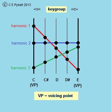
The spectrum for each of these 'unknown' notes must differ from its neighbours, otherwise we would merely be duplicating identically the same timbre across the keygroup. To do this we interpolate the amplitude of each harmonic in a pair of raw samples (now called voicing points) linearly across the keygroup in the manner illustrated in Figure 3.
Figure 3. Illustrating the linear interpolation of harmonic amplitudes across a five-note keygroup bracketed by two voicing points
This diagram depicts a five-note keygroup lying between C and E inclusive, and variations in the levels of three harmonics belonging to the known spectra of the two voicing points at C and E are shown as the coloured lines. In practice there could be many more harmonics, especially for stops such as reeds, such as the 62 harmonics shown for the Trompette pipe in Figure 1. Purely for the purposes of illustration, harmonic 1 (the red line) is shown with a higher amplitude for voicing point C than for E, whereas this behaviour is reversed for harmonic 3 (green line). Harmonic 2 (blue line) has the same amplitude at both voicing points. The problem is how to calculate the harmonic amplitudes for the intermediate 'unknown' notes C#, D and D# in the keygroup so that we can generate a gradually varying timbre or harmonic spectrum across these notes.
Because the lines joining the harmonics are all straight, we can use the equation of a straight line to work out their amplitudes for each of the 'unknown' notes C#, D and D#. This process is called interpolation, and because the lines are straight, it is known as linear interpolation. Curved lines could also be used, in which case this would become a so-called polynomial interpolator, but linear interpolation is simplest. Because the main object of the exercise is merely to generate a unique harmonic spectrum for each note so that its timbre differs slightly from its neighbours, linear interpolation is usually satisfactory. The use of interpolation not only produces the desirable small differences in timbre from one note to the next, but it also means the sound blends gradually from one voicing point to the next rather than changing abruptly in an unrealistic manner as you play notes up or down the keyboard.
As with AHI above, the interpolation process can be automated to some extent if not completely. By importing the spectrum files generated by the AHI algorithm for the voicing points into another computer program, a complete set of interpolated spectra for a given organ stop can be generated automatically. In fact a spreadsheet can be used instead of a specially-written program to perform the interpolation if desired, as the arithmetic involved is fairly simple. A screenshot of part of a typical Excel spreadsheet is shown at Figure 4.
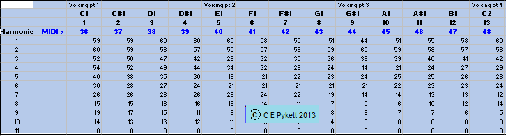
Figure 4. Extract from an Excel spreadsheet which performs linear interpolation of the harmonic values at the voicing points (Prestant 4', Pédale, Romanswiller)
The first octave (13 notes) of the pedal Prestant 4 foot stop at Romanswiller is represented in the figure. The harmonic amplitudes in decibels for the first four voicing points at C1, E1, G#1 and C2 are shown. Each pair of these bracket a keygroup of three additional notes. The numbers for the voicing point spectra were generated automatically in Step 1 using the AHI algorithm and saved in files which were imported into the spreadsheet. As soon as this is done, the interpolated spectra for all other notes in the various keygroups appear automatically. These numbers are now exported into the next stage of the process which generates the waveform samples for each note across the keyboard.
Should you wish to better understand the numbers which appear in this screenshot, be aware that the interpolation was performed on the linear harmonic amplitudes defining the voicing point spectra, not the logarithmic ones expressed in decibels which appear in the spectrum displays in this article. However the interpolated data were then converted back to decibels before appearing in the spreadsheet above. Interpolating the decibel values themselves would, of course, have produced different results. Either approach can probably be used however, as both deliver the desirable characteristic of a gradually changing timbre between voicing points.
Step 3 - generate the intermediate samples
A waveform can be produced from any spectrum - a set of harmonic amplitudes - using the process of additive synthesis. Sometimes this process is also called the Inverse Fourier Transform (IFT). Several programs exist for carrying out additive synthesis, and two well-known ones are KlangSynth (free) and AdsynDX (requires the purchase of a licence). Unfortunately KlangSynth, originally developed by Andreas Sims, is now elusive to obtain and it has not been supported for some years. AdsynDX, by Andy Bridle, ran under Windows XP and it also is no longer supported, though apparently it has been superseded by a Windows 7 version.
Some of these programs will accept a list of numbers in a file generated by my AHI spectrum analysis program or the interpolator spreadsheet just described, but I have to say that I find the type of user interface they employ is not ideally suited to generating the hundreds of wave files necessary for the purposes described in this article. To some extent this is nothing more than a reflection of my personal preferences, though I find it tedious to have to continually resort to mouse manipulation to achieve the end result for each and every sample. This article is to do with the problem of serious mass production of thousands of wave samples on an industrial scale, not simply fiddling about for ever with the odd one. Professional organ pipe makers and voicers cannot allow themselves this luxury any more than digital organ builders can if they want to achieve results before the universe ends! Therefore I have developed a suite of much simpler command line programs for carrying out additive synthesis. Like most of my software tools, they are written in C and one example is called AddSyn4. In my experience going back many years it is much slicker to use a command line interface than a pretty GUI, but in any case the program also performs vital additional processes such as automatically calculating loop points on the generated waveforms. This feature alone saves the untold time and effort which would otherwise be required to find them manually. The program will also optionally generate an attack transient if provided with the necessary data, and this aspect will be discussed in detail later. AddSyn4 accepts a string of numbers representing the harmonic amplitudes of a given note, such as those visible in the columns of the spreadsheet in Figure 4, and the numbers can either be typed in manually one by one (tedious but sometimes useful) or they can be read from a computer file (much quicker and less error-prone when generating large numbers of waveforms). Figure 5 shows a typical screenshot of the questions which AddSyn4 fires at you and the brief replies you have to give. As far as the user is concerned, the program executes instantaneously regardless of the number of harmonics in the synthesis.
Figure 5. Screenshot of the additive synthesis command line program 'AddSyn4'
To those unfamiliar with command line programs this prehistoric-looking picture will probably cause revulsion bordering on nausea. However a command line interface is widely used by seasoned computer users because it provides a fast, terse yet powerful means to control a program. More important than this, though, the programs can be used in what is called batch mode to run automatically hundreds of times, each time processing different data. Used in this way they are therefore well suited to streamlining the production of a sample set for a digital organ. To do this one writes a batch file which contains the scripts (detailed instructions) for running programs such as AddSyn4 over and over. The scripts tell the computer which programs to execute and in which order, and they contain all the answers in advance to the questions which the programs issue to the user, as in Figure 5 for example. Even the batch files themselves can be produced automatically or semi-automatically if one designs yet another suitable tool.
AddSyn4 provides a lot of options and it can be used in many ways. In the example shown it generated a sample in the form of a WAV file containing both attack transient and steady state sections. The partial/harmonic structures of the transient and steady state were provided in the two data files whose names appear in the dialogue. Suitable files are generated by the AHI algorithm for identifying harmonics described above. More detail on the difficult subject of transient synthesis is given later - for now, simply bear in mind that AddSyn4 is an instance of the tools used to implement the process.
Thus the simplest form of output from the additive synthesis program is a waveform segment with embedded loop points, representing the steady state waveform of a note at any given frequency (pitch). However (unless the program was instructed otherwise) it contains no attack or release transients, wind noise nor the small random perturbations in amplitude and frequency which characterise a real organ pipe while it speaks. Therefore these have to be 'added back' judiciously to some, but not all, notes if the entire stop (i.e. the collection of samples across the keyboard for a complete rank or stop) is to sound acceptable and realistic.
Using AddSyn4 together with the earlier processes described, a total of 923 wave samples were generated from the 265 raw samples in the original Romanswiller sparse sample set.
More often than not, the waveforms resulting from Step 3 cannot sensibly be used directly in a high quality digital organ. Apart from the steady state (sustain phase) speaking timbre, which is reproduced perfectly, all other aspects of the realism which organ pipes exhibit have been lost. These include transients, wind noise, and the slight randomness while a pipe continues to speak. Therefore these artefacts have to be recovered in some way and 'added back' to some of the samples. I strongly deprecate adding them back to all the notes because this makes a digital organ sound ridiculous. No real rank of organ pipes has the near-identical and pronounced chiff or breathiness on every note which one encounters on some commercial instruments. To keep this article to a reasonable length it is impossible to explain every last detail of how I recover all aspects of the realism, but the salient features of adding an attack transient will now be treated in some depth.
We shall consider how to incorporate an attack transient in one or other of the synthetic sample waveforms generated by additive synthesis in Step 3. Normally, a paradigm on which to base the transient to be modelled will exist in one of the raw samples used as voicing points, and if that sample was of sufficiently high quality then it could be used directly, complete with transient, in the target sound sampler. But if the raw sample was of low quality and it had to be re-synthesised using the method described above, or if its transient is also to be incorporated into another of the synthetic samples resulting from Step 3, then we need to invoke the following processes. Therefore the problem is to re-synthesise the transient having first determined its characteristics. Let it be said at the outset that the subject of transients is as much an art as a science, and what follows is based on decades of experience in electronic organ voicing. These techniques are presented not because they are necessarily better than any others or because no other approach is possible, but simply because they illustrate my preferred way of doing things which has evolved over many years. Note the need, yet again, for specially developed software tools.
The waveform of a typical attack transient might look something like that shown in Figure 6, which is the initial part of the Montre G#1 raw sample on the Grand Orgue at Romansiller.
Figure 6. Attack transient for the G#1 raw sample, Montre 8', Grand Orgue, Romanswiller
This transient lasts for around 500 msec before the pipe settles down to stable speech. At first sight it looks very complicated, and that's because it is. But to cut to the chase and without further ado, I have proved to my own satisfaction that one only has to define a ' start condition' for the transient, an 'end condition', and the time over which the transient evolves between the two. With this basic information and suitable tools it is possible to synthesise a wide range of realistic and satisfying transient sounds. I have come to the conclusion that using more complicated data and processes is seldom worthwhile in terms of the minor improvements obtained, if any.
The end condition is relatively simple - it is merely the harmonic spectrum of the speaking regime which the pipe exhibits during its sustain phase, and this has been discussed in detail above. Therefore the end condition is defined by applying the AHI (Automatic Harmonic Detection) algorithm to the sustain phase of the pipe sound. The start condition is more difficult, and here we have to call on some experience and judgement to discern what the data are trying to tell us. Expanding the transient in Figure 6 with a standard wave editor, one finds that it consists of two main parts, though for the sake of brevity this expanded trace is not shown here. The first part occupies the initial 40 msec or so of the sample, and it consists of a low-amplitude spit or noise burst as the pallet opens, thereby allowing the wind sheet to hit the upper lip of the pipe mouth. This noise then dies away rapidly. The second part follows on to occupy the next 450 msec or so. Here the transient proper begins to form, and by performing a spectrum analysis on this part of the transient we find it consists mainly of a dominant second harmonic, a characteristic which is common to the transients of many open pipes, especially those of Principal tone as this one is. This spectrum is shown in Figure 7.
Figure 7. Transient spectrum of the G#1 raw sample, Montre 8', Grand Orgue, Romanswiller (derived using a 2048 point analysis window starting 100msec from the beginning)
The analysis window was 2048 data points wide starting about 100 msec from the start of the waveform. Apart from the large peak at the second harmonic, little other discernible structure exists in the spectrum. However one has to be careful not to draw too many conclusions from this type of analysis. Because of the short time window (about 50 msec in duration), the spectrum resolution is only about 20 Hz because frequency resolution in any form of spectrum analysis, be it analogue or digital, is the reciprocal of the length of the segment analysed. This explains the broad peaks and the somewhat featureless look of the spectrum as a whole. Such problems are an inescapable part of transient analysis because if one tries to increase the frequency resolution, the necessary time window becomes so large that it encroaches on the sustain phase of the waveform. In such a case the structure of the transient itself would of course be submerged. The shorter the transient, the more difficult these problems become. Note that the frequencies of the harmonics in transients might differ slightly from those in the subsequent sustain phase of the sample, and they might not be exactly harmonically related either [4]. For these reasons they should really be called partials rather than harmonics. Therefore a synthesis tool is required which will generate the transient partials at any frequencies, and these might not always coincide exactly with the steady state fundamental and harmonics of the note being synthesised. However for the reasons just mentioned, spectrum analysis can only provide a rather coarse estimate of the partial frequencies comprising the start condition of the transient. Fortunately this is not actually a problem in practice because the ear itself performs a spectrum analysis, and it is therefore subject to the same constraints. It means that as a transient sound gets shorter, we are able to perceive progressively less of the frequency structure within it and how it evolves over time.
My additive synthesis program (AddSyn4) referred to previously will (optionally) generate a complete synthetic sample which includes both the transient and steady state components. To do this one supplies it with the spectrum of the transient as the start condition, that of the steady state phase as the end condition, and the desired evolution time of the transient (set at 450 msec in this case). For this example it then generated the transient waveform shown in Figure 8.
Figure 8. Re-synthesised transient waveform of the G#1 raw sample, Montre 8', Grand Orgue, Romanswiller - stage 1
Some of the characteristics seen in Figure 6 can also be discerned here - the transient evolves over about the same time, and the initial predominance of the second harmonic or partial gradually morphs into the harmonic structure which characterises the sustain phase of the sample. But the sample cannot be used in this form because it begins more or less at maximum amplitude rather than growing gradually. Therefore Figure 8 shows only stage one of a two-stage process. In the second stage we now have to overlay the correct attack envelope onto the sample. Thus stage 1 defines how the frequency structure of the transient varies with time, and stage 2 defines how the amplitude envelope varies. It is essential in my experience to have tools which provide the flexibility to adjust them separately.
The interactive facilities of a good sound sample editor can be used to implement stage 2. Most of them allow one to overlay an AHDS envelope onto the beginning of the sample (Attack/Hold/Decay/Sustain), and by applying this to the waveform in Figure 8 we get the result shown in Figure 9.
Figure 9. Re-synthesised transient waveform of the G#1 raw sample, Montre 8', Grand Orgue, Romanswiller - stage 2
The envelope parameters chosen were:
Attack: 200 msec (the time to reach the 'hold' phase) Hold: 100 msec (the time for which the amplitude is held constant) Decay: 80 msec ( the time for the envelope to decay to the 'sustain' level) Sustain: -8 dB (8 dB lower than the sample peak amplitude)
These were arrived at largely from measurements on the waveform in Figure 6, together with some empirical voicing adjustments made by ear. Although there are some visible differences between Figures 6 and 9, the re-synthesised transient nevertheless has the essential richness of the original and it sounds virtually identical.
In the expanded Romanswiller sample set containing 923 samples, 133 of them have attack transients. Most of these have unique properties - they are by no means the same. For example, one should not apply a transient which is characteristic of an open flue pipe to a stopped one. The majority were added as just described, though a few also existed on those raw samples which were useable directly. Overall, this means about 15% of the samples have perceptible transients, which to my mind feels right and what one might find on a typical pipe organ. On average it implies that about 9 notes per stop have noticeable transients. In practice, some will have more and others less. The characteristics of all the transients were restricted to the outcome of an analysis of those in the original sparse sample set - none were imported from other organs.
Although it is possible to automate transient generation to some extent, this is an area where much attention to detail in the voicing and tonal finishing of the instrument is necessary if it is to sound realistic. In my opinion, on a French organ of this era there should not be too many transients nor should they be too obtrusive, yet those which do exist should be lifelike and they should enhance the overall articulation without dominating it. Enhancing colour and articulation were the dominant aspects here rather than emphasising spit and chiff for their own sake. I dislike those digital organs which seem to say "I am using a clever sound engine which can reproduce transients, and I am not going to let you forget it"!
This subject will not be discussed in detail for reasons of brevity. It relates to the small variations in amplitude and frequency which characterise an organ pipe while it speaks in its steady state (sustain phase) regime, and these can be imposed on the samples generated by the AddSyn4 additive synthesis program. Provided the sample duration is long enough (which the user can specify) the program will then apply small random changes in amplitude and/or frequency to randomly-chosen segments of the synthesised waveform. Its amplitude envelope then takes on the somewhat 'ragged' appearance of that of a real organ pipe.
Likewise, this subject will not be covered in detail. Noise which it is desired to retain on a waveform, such as the 'breathiness' of pipes while they speak, is difficult to handle in sound samplers because it makes the samples virtually impossible to loop successfully. This is not surprising because one is trying to loop two completely different signals simultaneously. One of the signals is largely deterministic, meaning its behaviour is mathematically predictable at all times. This is the waveform without any imposed noise, and such signals can be looped fairly readily. However the other signal, the noise, is random and it cannot be predicted at all. Even if loop points can be found on the composite waveform which do not result in audible clicks, and this is rare, the repetitive looping over what should be a continuous random signal segment often enables the ear to detect that something is amiss. Our ears and brains are astonishingly clever and it is difficult to fool them. For example, a repetitive 'swishing' sound is commonly detectable as the sampler loops repeatedly over the same segment of the signal plus its noise.
There are basically two ways around this. One is to use noisy samples of such a length, e.g. five seconds or more, that looping will seldom be invoked in normal playing. The other is to add suitably-engineered noise from an independent noise source whenever the sample (without noise) is keyed. This can be done fairly easily in the rendering engine itself as the simulated organ is played, though it might consume additional polyphony.
The Expanded Romanswiller Digital Organ
Using the expanded sample set derived as above, the Romanswiller simulation was modified and enlarged in other ways as follows:
These changes do not detract from the historicity of the instrument because at the time it was sampled it had lost much of its authenticity in any case (see the PDF file outlining its history [2]). Instead they have turned it into a simulation of what a pipe organ builder might make today if asked to create a pastiche organ with a strong French flavour before Cavaillé-Coll came on the scene. It makes a useful and attractive addition to the range of Prog Organ simulations, and it gives considerable satisfaction to the player.
The following mp3 tracks might give some idea of how the instrument sounds.
Articulation with a mezzo-forte flue chorus:
The augmented pedal organ:
Full organ without manual reeds:
Another pedal solo from the Orgelbüchlein:
It is also interesting how Young's temperament copes with these keys (C minor, A minor, D major and F major respectively) as well as the modulations within the pieces. It is a very agreeable temperament designed by a polymath. One of the reasons for developing this simulation was so that I would have an instrument available which speaks in this temperament.
This article considered the problem of generating a complete sample set for a digital sound sampler, comprising an independent and different sample for each note, from sparse or incomplete data. The common technique of stretching a sample across a range (keygroup) of notes was not used because this results in an identical timbre or tone quality for each note of the keygroup. Moreover, that timbre then changes abruptly from one keygroup to the next. These deficiencies sound artificial and unsatisfactory. Instead, the approach here used all raw samples directly in the sampler, and in addition reference spectra were also derived from them. Interpolation from the reference spectra was then performed to generate a unique harmonic spectrum for each of the 'missing' samples, which were then generated using additive synthesis. The problem of restoring the necessary realism to the synthesised sounds was illustrated by describing in detail how an attack transient can be analysed and then incorporated in a sample as it is synthesised.
The article emphasised the need for special purpose software tools, not only to implement some stages of a rather complex process in the first place, but to realise them in a time-efficient manner. These tools were deliberately written as stripped-down command line applications which are suitable for batch-processing the hundreds or thousands of samples needed for a high quality digital organ. Examples of the operations carried out include automatic harmonic identification, interpolation, additive synthesis, calculation of loop points and some aspects of transient generation.
These techniques enable a complete sample set to be built from a sparse one using features of both sampling and additive synthesis - the real samples can be used directly in a sound sampler, and they are also analysed to enable the remaining samples to be generated by interpolation followed by additive synthesis. This arguably makes the best of both worlds. Thus all samples in the complete set are based directly on real pipe sounds, which they would not be if they were derived using an approach such as physical modelling.
The widely-available sparse sample set of the Stiehr-Mockers organ at Romanswiller in France by Joseph Basquin was used to illustrate the points made in the article. The 265 original samples were expanded to 923, of which 133 had attack transients.
I should like to acknowledge the service rendered to the virtual pipe organ community by Joseph Basquin and his colleagues in making the Romanswiller samples so freely available. Use of the samples is in accordance with the originator's licence conditions and will remain so.
1. See Re-creating Vanished Organs, an article on this website, C E Pykett, 2005.
2. At the time of writing (February 2013) the Romanswiller organ samples can be downloaded from www.jeuxdorgues.com/?lang=en.
A description of this interesting organ in an English translation by myself is also available as a PDF file on this site (download).
3. The following articles elsewhere on this website relating to digital organ voicing are listed in date order with the most recent first:
4. Transient formation in organ pipes is covered in detail in the article A Second in the Life of a Violone, C E Pykett, 2005.
|