


|
|
|
The physical modelling of organ flue pipes - a complete picture
being
The Compleat Physical Modeller
by Colin Pykett (with apologies to Izaak Walton)
Posted: 26 August 2013 Last revised: 16 February 2017 Copyright © C E Pykett 2013-2017
Abstract. Physical modelling is the latest technique for the digital simulation of musical instruments generally, and it is also found in a minority of digital organs and organ synthesisers. However there is almost no literature available to assist the non-specialist in coming to grips with what is involved, its strengths and its limitations. As the underlying concepts are far from new, this article will describe how an organ flue pipe can be modelled using physical principles which became well-established three decades or more ago. Models of the oscillatory mechanism of the air jet at the pipe mouth, the resonating action of the pipe body and how the sound from the pipe emerges to form a sound wave in the surrounding atmosphere itself are all described. Thus the article presents a complete picture as its title indicates but without recourse to mathematics or complicated physics. This makes it unique in both respects - completeness, and its accessibility to a broad readership.
The overarching problem of physical modelling lies in its necessary reliance on the approximations which are identified in this article. Some of the processes involved in pipe speech are imperfectly understood, or they involve intractable mathematics which is not well suited to real time synthesis on small computers. Even if this were not so, all problems in aerodynamics are fundamentally insoluble at a detailed, rigorous level because the underlying Navier-Stokes equations cannot be solved either. The situation does not signify a total impasse by any means, but it implies that physical modelling is a better synthesis technique in some cases than in others. For instance, the simulation of every pipe in a specific organ is probably best realised using sampled sound synthesis, because this gets round the approximation problem simply by recording the actual pipe sounds directly. It is difficult to argue that the sounds of real pipes can be improved by any form of modelling, so when the samples are subsequently replayed by the performer one has a more or less exact reproduction of the sounds of the original instrument. However there are inflexibilities inseparable from any sample set, such as that related to the fixed microphone position at which the samples were recorded. These inflexibilities do not apply as strongly to physical modelling because the range of parameters which can be adjusted in a good model allow spatial effects, for example, to be modified at will. Thus the simulated listening position can be adjusted within wide limits. On the other hand, the approximate nature of physical modelling means that it cannot approach the sound of a particular pipe at a particular listening position as closely as does sampled sound synthesis. Thus the issue boils down to the alternative between simulating particular pipes exactly by sampling their sounds, or simulating a wider range of pipes approximately using physical modelling. Both techniques have their place, and ultimately the choice between them must lie with the customer. Therefore it is hoped this article might illuminate the issues which need to be considered regarding physical modelling.
Contents (click on the subject headings below to access the desired section)
Jet drive mechanism of the flue pipe
Harmonic generation - the nonlinear oscillator
A case study - the Viscount digital organ
Physical modelling synthesis is the most recent of the three main methods used for simulating musical instruments, the other two being sampled sound synthesis and additive synthesis. Sampled sound instruments contain many digital recordings (waveform samples) of the actual sounds of real organ pipes. Those using additive synthesis build up the sounds in real time as the instrument is played, harmonic by harmonic, thus it is a step towards modelling the sounds as opposed to replaying pre-recorded waveform samples on demand. Physical modelling goes further in that the sounds are generated from scratch in real time using equations and computer algorithms, as no previously-stored recordings or tables of harmonics are involved. Although the technical basis underlying physical modelling - the equations and algorithms - had become well established three or more decades ago, its commercial appearance had to await the availability of today's sufficiently cheap and powerful computer technology. As additive synthesis is now fading from the scene, the result is that the majority of digital organs still use sampled sound synthesis, a technology whose roots go back to the 1970s. However physical modelling is being applied increasingly widely in digital music more generally, where it is well matched to simulating other instruments such as pianos, orchestral instruments and even the human voice.
There were two motivations for writing this piece. Firstly there is almost nothing in the literature which explains physical modelling at a level which non-specialists can comprehend, and secondly much of what is available fails to embrace all aspects of modelling an organ pipe. For instance, we find much attention paid to the physics and mathematics of the oscillating air jet at the mouth of a flue pipe, yet there is sometimes less consideration of the equally important details concerning the resonating tube sitting above it. Therefore it is hoped this article will remedy both deficiencies by describing physical models at a level which can be readily visualised, as well as covering all the pertinent acoustic mechanisms of the whole pipe. To keep its length within reasonable bounds many references are given to material elsewhere on this website and in the wider literature, rather than attempting to explain everything from first principles. This might make the article inconvenient to assimilate but there was no practical alternative.
An overriding factor which needs to be kept in mind is that physical modelling can only deliver an approximation to the sound of a real organ pipe at the current state of the art, though this criticism is not exclusive because other simulation methods all have their own limitations. The issue arises here because aerodynamic systems such as organ pipes cannot be modelled exactly, therefore their sounds cannot be simulated exactly either. Achieving this would require solutions to the Navier-Stokes equations governing air flow, and these have remained resolutely insoluble since they were formulated in the nineteenth century - a million dollar prize is yet to be claimed. Therefore, although the mathematical basis of the various physical models one finds in the literature invariably looks complicated, and that's because it is, the models nevertheless represent only a simplified approach to reality. It is true that more exact solutions can be achieved nowadays using what is called CFD (computational fluid dynamics) on powerful computers, but to date little headway has been made by applying it to organ pipes. Therefore considerable reliance has to be placed on the 'simplified' (!) mathematical approach, together with the results of experiments which are then incorporated in one way or another into the models. So the models are not only simplified but some of them also contain a good proportion of empiricism and heuristics - kludges, not to put too fine a point on it. The consequential limits imposed on the fidelity of the simulated sounds are described as they arise throughout the article. But have no fear, we discard the mathematics entirely here.
Much of the background relevant to this article can be found in others on the site, thus deferring the need to delve frequently into the wider literature. The fundamental processes which result in a flue pipe emitting sound are outlined at a simple and generic level in reference [1]. These are then illustrated with respect to the three special cases of flute [2], principal [3] and string pipes [4]. Some aspects of physical modelling were addressed in [5], though this only outlined how the resonator can be modelled using the technique of waveguide synthesis rather than dealing with the pipe as a whole. Thus sound generation at the mouth was not described in that article, a deficiency which is remedied here.
If you are unfamiliar with how flue pipes speak, in particular their dependence on the intimate coupling between sound generation at the mouth and resonance in the air column, then reference [1] should be consulted before reading further.
Jet drive mechanism of the flue pipe
By about 1985 details of the oscillator or sound generation mechanism in a flue pipe had become more or less finalised and widely accepted within the physics community, and a detailed review can be found in reference [6] (page 503 et seq). Like much else in the physical modelling literature, this book was written for professional physicists as it demands not only a graduate level knowledge of physics but of mathematics as well. This is not a criticism, but it does underscore the need for an article like this one. So here goes.
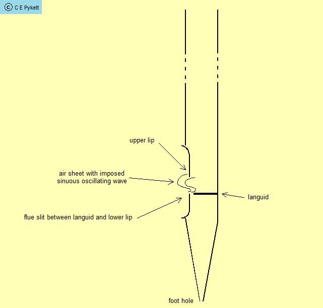
Figure 1. Structure of a typical flue pipe
Consider the structure of a typical flue pipe, as shown in Figure 1. It is intuitively obvious that the air sheet at the mouth must oscillate in some way because sound is generated by the pipe when air issuing from the flue hits the top lip. However the details of exactly how it oscillates are pivotal to the successful modelling of the pipe, and it is this we shall now explore. Because the flue is a narrow slit, air emerges from it in the form of a equally narrow sheet like a curtain across the mouth of the pipe. Initially it travels at a speed around 35 metres per second (nearly 80 mph) for moderate blowing pressures around 75 mm of water (about 3 inches), but note that this refers to the sub-languid pressure (that within the pipe foot just below the languid) rather than that within the chest on which the pipe stands. The distinction is important because it is overlooked by some authors, and it arises because the foot holes of almost all flue pipes are deliberately constricted so that their loudnesses can be regulated by the voicer. Enlarging the foot hole increases the loudness and vice versa. In a metal pipe the hole size is varied by working the soft metal, whereas in a wooden one wedges or plugs can be inserted or removed. A foot hole capable of imposing a flow reduction on the air passing through it implies that its area needs to be comparable with that of the flue slit itself. Even so, quite large foot holes can still reduce the pressure at the flue by a significant amount - one having an area three times that of the flue will reduce the sub-languid pressure by typically 10%. Another reason for modelling carefully the pressure reduction by the foot hole is the effect it has on the attack and release transients of the pipe, a subject treated later on [7].
If there were no resonating tube or upper lip above the languid, the pipe could not speak because there would be no pipe as such. In this circumstance the sheet-like jet would simply slow down rapidly as it travelled further away from the flue. It would also broaden from its initial narrow width imposed by the slit, and eventually it would dissipate into eddies in the atmosphere at large. However, by means of a suitable flow visualisation experiment (e.g. one using smoke-laden air) it is possible to demonstrate the instability of such a jet by perturbing it some way. Simply by poking a pencil into the air sheet at some point, the relatively ordered character of the initial jet will in most circumstances become wildly disturbed downstream of the obstruction. Not only might eddies form rapidly, but these and other perturbations would grow quickly with increasing distance. This inherent instability of the jet and its ability to amplify a disturbance are important when we now examine what happens when an organ pipe speaks.
While an organ pipe is speaking a strong acoustic field exists at its mouth. This results from the pressure impulses travelling up and down inside the pipe as described in [1], and as they appear at the mouth they alternately push and pull on the air jet. The jet obviously cannot move at the point where it emerges from the flue, but above this it is progressively deflected in and out of the mouth by the sound impulses. Together with the unstable nature of the jet and its tendency to amplify disturbances, the net effect is that a wave-like motion begins to travel upwards with the jet, getting larger in amplitude the further it goes.
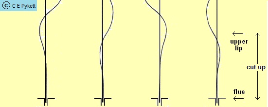
Figure 2. Illustrating how an oscillating air jet flips repeatedly across the upper lip of the pipe
This is illustrated in Figure 2 which shows the shape of the upwardly-travelling wave on the jet at several successive instants. The perspective of this sketch is the same as that of Figure 1 - we are looking at a cross-section of the pipe mouth with the long dimension of the flue slit coming towards us out of the plane of the diagram. The curvy lines represent the central plane of the oscillating air sheet, which broadens and loses speed as it progresses upwards from the flue (the broadening is not apparent in this diagram). The speed of the wave is about half that of the air in the jet itself, which means it travels at much less than the speed of sound (which is about 344 metres per second). As the frequency of the wave is the same as the fundamental frequency of the pipe, this means the length of the wave measured on the jet is much smaller than the wavelength of the sound emitted by the pipe into the atmosphere, because wavelength equals speed divided by frequency. Therefore the short distance between the flue and the upper lip (called the cut-up) represents an appreciable fraction of the wavelength of the travelling wave, so by the time it reaches the lip the tip of the jet flips sinusoidally into and out of the pipe as the phase of the oscillation at the lip changes continuously with time. While the jet is inside the pipe it injects a puff of air into the air column of the resonator, the pressure and speed of which maintain the speech of the pipe by compensating for energy losses in the resonator [11]. The shape of this impulsive injected waveform also defines the harmonic spectrum generated at the mouth, a spectrum which is then modified by the resonating properties of the air column. These matters are discussed later.
The effect of varying cut-up height is one of the more successful outcomes of physical modelling to date as far as voicing adjustments are concerned. As the cut-up increases, the speech of the simulated pipe should get weaker until eventually its pitch should jump abruptly to (approximately) the octave above, whereupon it should then speak with a thin quavery sound. This applies to an open pipe; for a stopped one the effects are different. Such behaviour is commonly observed in practice with badly voiced pipes if the wind pressure is too low for the cut-up. It occurs because progressively more half-cycles of the wave on the jet are able to interact with the the resonator until they begin to preferentially excite its second natural resonance rather than the first (an example of what is called mode-switching). The modelled pipe can be returned to normal speech by leaving the cut-up as it is but increasing the simulated wind pressure (though the harmonic structure of the sound should not be quite the same as previously if the model is a good one). This occurs because increasing the blowing pressure increases the jet speed and thus the travelling wave speed, thereby increasing its wavelength to better match the higher cut-up. Demonstrations of these effects can be quite convincing in a successful physical model. Indeed, if they do not occur then the model needs improving.
Aside from cut-up and sub-languid wind pressure, the other main adjustments available to a voicer are lip sharpness, lip offset relative to the flue, flue width, languid height, the fitting of ears and beards, foot hole area and nicking. Unfortunately it is a Herculean task to conceive of incorporating all these into a physical model which can only call on approximate mathematical formalisms at best. Nicking is particularly difficult to simulate because it encourages immediate turbulent flow at the languid, and turbulence (like much else in aerodynamics) resists attempts to model and understand it in detail. The physics of all these voicing adjustments has been described at a qualitative level elsewhere on the site in reference [4] (see the section entitled The Physics of Voicing).
A further problem with the air jet model just described relates to its implied symmetry. The oscillating sheet was assumed to move in and out of the pipe as though conditions are identical each side of the mouth, whereas this is obviously not the case. While it is transiting from inside to outside the pipe, the sheet moves virtually unconstrained into the almost free acoustic field of the open atmosphere (neglecting the effects of ears or beards), but when moving back into the pipe it is travelling into an enclosed space which is certainly not a free field. It can therefore be affected, for example, by air pressure reflections from the pipe wall opposite the mouth and these will vary depending on mouth size, pipe scale and whether the pipe is rectangular or cylindrical [8]. The jet also injects air into the pipe, thus if the pipe is stopped the excess air can only escape via the mouth, so the jet has to work against a unidirectional outflow from within. Then there are the imponderables associated with the interaction of the jet with the standing wave inside the pipe, whereas there is no such interaction outside. For example, it is not straightforward to establish the relative theoretical importance of air flow from the jet (kinetic energy) versus its pressure (potential energy) as it gives up energy to maintain the internal standing wave [11]. All these factors mean that yet further approximations have to be forced into the model so that it better explains reality. The difficulties have been acknowledged by some authors who wrote that current understanding and modelling practice "conceals a great deal of ignorance about the aerodynamic details of the system" [6] (page 515).
Harmonic generation - the nonlinear oscillator
One often sees the term 'nonlinear oscillator' in the physical modelling literature, and here we investigate what it means. It is related to the ability of the oscillating system of a musical instrument to generate a spectrum of harmonics, which of course play an important role in defining its tone colour or timbre.
It is at first sight a curious fact that the tip of the air jet sweeping in and out of the pipe across the upper lip moves almost sinusoidally back and forth, yet the jet generates a more or less extensive harmonic series which is then imparted to the resonating air column. But a sinusoidal oscillator only generates a single frequency - its frequency spectrum consists of only one harmonic - and the mathematics describing such oscillators is called 'linear'. So how do the other harmonics appear? It might be helpful to illustrate the situation first with an analogy from electronics. If we have a sine wave oscillator or signal generator, which only has a single harmonic, we can easily make it generate lots more of them by simply increasing its amplitude by a large factor. When the peak amplitude of the sine wave hits the supply voltage limits of the circuit it cannot increase any further, and then the smooth sine curve suddenly turns into a waveform with flat portions at the top and bottom of the voltage swing. By continuing to apply more and more gain (amplification), eventually the former sine wave will turn into a square wave, and this has a long retinue of odd-numbered harmonics. The mathematics describing the modified circuit, consisting of a sine wave oscillator followed by a high gain amplifier, is now termed 'nonlinear'. Thus the modified oscillator is likewise called a nonlinear oscillator.
No non-electronic musical instrument generates a pure sine wave even though the oscillating element itself might move sinusoidally, but the actual mechanisms differ from one instrument to another and the electronics analogy therefore cannot be taken too far. Some instruments are more difficult to visualise than others, but the free reed as used in harmonicas, accordions and harmoniums is one of the simpler examples. Here, the reed tongue itself oscillates sinusoidally within a close-fitting aperture in the mounting frame but it generates a sound which is far from a simple sine wave with just one harmonic. In fact it is often difficult to tame the generated spectrum from a free reed so that there are not too many harmonics in its sound, which is frequently coarse and unpleasant. The reason why the sinusoidally-oscillating reed generates the harmonics is because the windway, the geometric aperture covered and uncovered by the reed in its frame as it moves, varies grossly non-sinusoidally with time. Therefore the puffs of air which get through the frame from the bellows have a pulse-like shape with many harmonics.
Now for the oscillating jet at the mouth of an organ pipe. Let us look first at the air speed profile across the thickness of the jet, illustrated in Figure 3.
Figure 3. Illustrating how the air speed profile across the jet changes with distance from the flue
Again we retain the same viewing perspective as before by looking at a (magnified) cross-section of the pipe mouth with the long dimension of the flue slit coming towards us. At first, air issuing from the narrow flue moves at virtually the same speed across the thickness of the jet, leading to a rectangular speed profile just above the flue. However the jet broadens and slows down as it propagates upwards as a result of the drag it experiences against the stationary air of the atmosphere, as shown by the dotted lines in the sketch. Because the air inside the jet is subjected to lower drag than that at the outer edges, the speed profile evolves to a smoother curvy form higher up the jet. This smoothing effect becomes more pronounced the higher up the jet we go. The evolution of the smoothing progression also depends on the sub-languid wind pressure, flue width and whether the languid and/or lower lip are nicked. If nicking is used the depth and density of the nicks (the number of nicks per centimetre) are also important.
The physical model must accommodate all these factors if an accurate jet speed profile is to be simulated, because the speed profile at the upper lip is critical in determining the harmonic spectrum of the waveform which is delivered to the resonating air column of the pipe. To see how the harmonics are generated, consider the tip of the oscillating jet as it is about to move across the upper lip into the pipe body.
Figure 4. Typical air flow rate waveform into the pipe
Figure 4 is a sketch of what the air volume flow rate injected from the jet into the pipe body might look like for a typical speed profile across the jet. Let T be the oscillation period of the wave on the jet, which is the same as that of the fundamental frequency being sounded by the pipe. Then at time T = 0 in the diagram the jet begins to enter the pipe as it moves across the upper lip from outside, at T/4 it has fully entered the pipe, and by T/2 it has left the pipe again and is moving back into the external atmosphere. After a complete oscillation period has elapsed the jet begins to re-enter the pipe once more at time T. Therefore the jet is injecting pulses of air into the pipe once per cycle. (There will also be an outflow of air from the pipe to prevent pressure building up internally, and this will modify the waveform in a manner which depends on whether the pipe is open or stopped. However the way this affects the waveform is not shown in the diagram). It is obvious that this pulse-type waveform is far from sinusoidal, even though the tip of the jet moves sinusoidally back and forth across the lower lip. Thus a linear oscillator has been converted into a nonlinear one, as happens in many musical instruments, and the non-sinusoidal waveform means it contains many harmonics. It is not difficult to see that the shape of the injected pulses will depend on the shape of the speed profile across the air jet, because a profile with sharply-defined rise and fall times (such as the rectangular profile close to the flue) will result in sharper pulses and vice versa. The width of the air jet at the upper lip also plays a part in that a narrow jet at this point will result in shorter pulses than a wider one. All this explains why a low cut-up (where the jet width at the upper lip is narrow) results in the pipe speaking with many harmonics, whereas a higher cut-up reduces the number. We should note at this juncture that the model should incorporate yet another parameter, the sharpness of the upper lip, because this also has an effect on the generated pulse width. This makes clear the result of broadening the upper lip, for example by leathering it, because the generated pulses are then less sharp and so they contain fewer harmonics.
The pulse train sketched in Figure 4 is symmetrical in that the pulse width equals the time between pulses (T/2 in both cases). It can be shown that such waveforms contain odd-numbered harmonics which are stronger than the even-numbered ones. The reason for this should become clearer if, purely for purposes of illustration, we replace the smooth pulses drawn in the diagram with rather unrealistic sharp-edged ones, as in Figure 5.
Figure 5. Symmetrical and asymmetrical pulse waveforms
The left hand part of the diagram is the same as that in Figure 4 except that we have replaced the smooth pulses with rectangular ones, thus the waveform has now become an ordinary square wave. It is well known that this contains only the odd-numbered harmonics. Although the even-numbered harmonics are never completely absent in a real organ pipe because the waveform injected into the pipe is never exactly a square wave, this might help in understanding why they can nevertheless exist with lower amplitudes than the odd-numbered ones. In fact the voicer can encourage this by adjusting the injected waveform to be as symmetrical as possible. This occurs when the lip offset from the flue is near to zero, in other words when the upper lip lies more or less exactly above the flue slit. This geometry arises automatically for most wooden pipes because of the way they are made, whereas the lip in a metal one can be pulled in or out slightly to achieve the desired condition. Flute stops are often voiced with a zero lip offset because it endows them with an attractive hollow, somewhat 'woody', tone even when the pipes are open rather than stopped (the presence of a stopper reduces the even harmonics even further).
This voicing condition is highly undesirable for principal and string toned stops however, which must have a complete harmonic series containing both odd and even harmonics. This is achieved by making the injected waveform asymmetrical as shown on the right hand side of Figure 5. Here the time spent by the jet inside the pipe is less than than the time it spends outside, leading to a pulse train having narrower pulses than before. An asymmetrical rectangular pulse train has both odd and even harmonics in its spectrum (though there are missing harmonics elsewhere, a feature we shall not pursue further here). To achieve the asymmetry the voicer deliberately introduces a lip offset by pulling the lip out of the pipe, or s/he deflects the air jet at an angle towards the upper lip by pulling up the languid.
The major issues involved in jet formation and harmonic generation have now been covered above in a qualitative and illustrative fashion, but a physical model must be able to handle all of them quantitatively. To summarise, the model must derive the air speed profile of the jet at the upper lip as a function of input parameters which include foot hole area, sub-languid wind pressure, languid height relative to the lower lip, flue slit width and length, and whether the languid and/or lower lip are nicked. If present, nicking must be further parameterised in terms of the depth, shape and density of the nicks. The mouth itself must be defined in terms of width, upper lip shape (straight or curved), upper lip sharpness, cut-up, lip offset relative to the flue, and the dimensions and positions of ears and beards. Injected pressure and flow rate waveforms delivered to the air column must then be derived as a function of all these parameters, and the energy contributions of both (pressure and flow) to the steady state speaking regime of the pipe must be obtained [11]. All this adds up to a formidable task. To set it against an easily understood mathematical yardstick, the mouth of any organ pipe is usually rectangular, yet there is no simple equation describing a rectangle as there is, say, for a circle or an ellipse. Unfortunately pipe mouths are seldom circular or elliptical, however. So if it is difficult to describe something as basic as a rectangular mouth shape before one can even begin, should we be surprised that physical modelling has to fall back on approximations elsewhere when the going gets tougher?
The body of the pipe above the mouth acts as a resonator by supporting standing waves in the air column. The way this happens is outlined in reference [1], and the processes are also represented in terms of an acoustic waveguide in [5]. As both of these references are to articles elsewhere on this website they can be consulted readily, so they will not be discussed further here. Waveguides are used in some physical models to simulate sound waves travelling along strings or within air columns, and they are examples of time domain models. While we could continue by pursuing the details of a refined waveguide model at this point, it is more appropriate to use a frequency domain representation of the air column. This is because, although we started by considering the wave on the air jet in the time domain, we then moved into the frequency domain when discussing its harmonic structure.
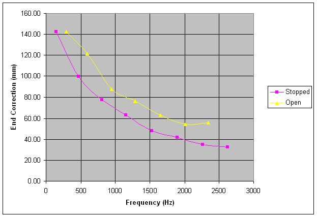
A frequency domain representation of an enclosed air column, such as that of an organ pipe, means we have to model its natural resonant frequencies. These are quite different from the harmonics the pipe emits when it speaks because the natural frequencies exist regardless of whether the pipe is being blown or not, although we never hear them as such. They are properties purely of the enclosed air. The most important feature regarding pipe resonances is that each natural frequency has an end correction which is numerically different from all the others. The lowest natural frequency has the largest end correction, with the higher-order resonances having successively smaller ones. This behaviour is illustrated in Figure 6 for both and open and closed pipes.
Figure 6. Variation of end correction versus natural frequency for a stopped and open pipe [9]
These measurements were made by me on an actual organ pipe as described in reference [9], and they lead to a second important feature which is that the natural frequencies are mutually anharmonic (i.e. they are not harmonically related). This arises because the first resonance has by far the largest end correction as Figure 6 shows, which means that the pipe seems longest for the first resonance in an acoustic sense. Because of the pronounced nonlinearity of this graph, there is no simple relation between the frequencies of the natural resonances as there is for the harmonics in its sound. Whereas the harmonics emitted by a pipe when blown are exact integer (whole number) multiples of the fundamental frequency, the natural frequencies cannot be predicted simply by knowing the frequency of the lowest because they deviate considerably from harmonicity [10].
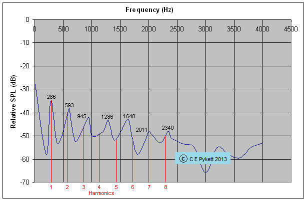
The natural frequencies of the open pipe whose end corrections are plotted as the yellow curve in Figure 6 are shown in Figure 7, together with the positions of its harmonics marked along the frequency axis by the red lines.
Figure 7. Measured natural frequency spectrum of an open pipe [9]
The first harmonic of this pipe when speaking coincided exactly with its first natural frequency at 286 Hz, but the correspondence between the other harmonics and resonances is progressively lost for the higher frequencies. (Although a close match might seem to exist for the 7th harmonic, the effect is fortuitous because the correspondence is actually with the 6th - not the 7th - natural frequency). This graph illustrates perfectly the widespread confusion which exists about the natural frequencies of organ pipes. Frequently one finds statements in the physical modelling literature suggesting that the natural frequencies of a pipe are 'nearly harmonic', yet the data here show that this is certainly not the case. Their anharmonicity is marked, and the effect is clarified further in Table 1 below.
Table 1. Discrepancy between the harmonics and the natural frequencies of an open pipe
It can now be seen clearly that the natural resonances lie progressively sharp of their corresponding harmonics, with the frequency discrepancy reaching 17% for the higher resonances. Put another way, this means the two highest resonances are around 272 cents (nearly three semitones) sharp of their corresponding harmonics, which is why the 6th resonance nearly coincides with the 7th harmonic of this particular pipe as noted above. Not all physical models are capable of modelling this singular behaviour successfully. The pipe under discussion here was an ordinary one pulled from an organ, yet its end correction at the fundamental frequency was equal to some 31% of its physical length. End corrections of this magnitude are typical for organ pipes, but they cannot be predicted successfully unless the pipe is modelled as a 3-dimensional cavity resonator rather than using the common and simplistic 1-dimensional approach. Only a 3-dimensional method can handle the pronounced variation of end correction with pipe scale (the relation of cross-sectional area to length) and with pipe shape (square, rectangular, triangular or cylindrical). Also the so-called end correction phenomenon is actually due to air masses surrounding the mouth and top of the pipe into which the acoustic energy is initially coupled, and within which the sound first propagates as a near-field wave before evolving into a far-field plane wave in the auditorium at large. Modelling this coupling demands a 3-dimensional approach comparable to that used for modelling loudspeakers mounted in enclosures. Unless the end correction and its variation with frequency can be modelled for a pipe of given dimensions, generating results which correspond closely to those shown in Figure 6, it is impossible to derive the frequencies, amplitudes and Q-factors of the natural resonances.
Computing values for these parameters is essential if the effect of the natural resonances on the harmonic series generated by the air jet is to be modelled, because the natural resonances act as an asymmetrical comb filter applied to the harmonics. The filter is asymmetrical because the 'teeth' of the comb are not equally spaced in frequency. It should be reasonably clear from Figure 7 that the way the natural frequencies affect the harmonics, by amplifying or attenuating some more than others, depends on where the natural frequencies lie relative to the harmonics on the frequency axis, and the sharpness and height of each peak. These matters are discussed more fully in reference [9]. Incidentally, the emphasis placed here on natural frequencies does not mean that a frequency domain model of the resonator must always be employed. Time and frequency domain models are equivalent in all respects, the choice between them depending on issues such as the relative complexity of the mathematics and the preferences of the modeller. Therefore a suitable time domain model such as an acoustic waveguide can be used in principle. However it would be far more complicated than the simple one discussed in reference [5], which was intended only to illustrate some basic ideas about waveguide synthesis.
Summarising resonator effects, a standing wave inside the pipe is generated at the fundamental frequency it emits when speaking. The fundamental is considerably flat (lower in frequency) compared with what one might expect from the pipe length because of the significant end correction at this frequency, and its frequency is equal or very close to that of the first natural resonance of the pipe. As well as setting up a standing wave, the air impulses travelling up and down in the air column at the fundamental frequency also result in the formation of a wave on the air jet at the mouth having the same frequency, and in turn the standing wave is maintained by taking energy from the jet. Harmonics of the fundamental exist at exact integer multiples of the fundamental frequency, but they are subjected to spectrum shaping by the action of the anharmonic natural resonances of the pipe which constitute an asymmetrical comb filter. The anharmonicity of the natural resonances arises owing to the variation in their end corrections with frequency. It follows that a physical model must predict the end correction accurately for a pipe of given dimensions, and its variation with frequency, so that the natural resonances can be defined in terms of their frequencies, amplitudes and Q-factors. This requires the pipe to be modelled as a 3-dimensional resonator rather than relying on the over-simplified 1-dimensional model which is commonly used.
Modelling the myriad subtleties of attack transients in a way which convinces the ear is difficult. A given pipe can emit a wide range of evanescent sounds as it comes onto speech, varying from none at all to the prolonged and almost painful way a string pipe can struggle to attain stability. Between these extremes lie the assorted harmonics one sometimes hears fleetingly as the note is keyed, such as the second and/or fourth harmonics often emitted briefly by principal pipes or the 'chiff', whispers and whistles at the third, fifth or seventh harmonics of some flutes. A skilful voicer can encourage or suppress much of this behaviour using several tricks of the trade, of which one is adjusting the foot hole to alter the point at which the pipe sits on the curve defining its speaking frequency versus sub-languid wind pressure. If the pipe lies near to the point at which it overblows to a harmonic, it will have a tendency to emit a more pronounced transient than if it sits at a pressure well below this threshold. Therefore this is another reason why it is important to include the effect of the foot hole in a physical model [7]. Other adjustment techniques include nicking the languid and/or lower lip, and adding or adjusting the beards applied to string pipes. Other factors are not within the voicer's control, such as the type of action employed to open the valve at the pipe foot. An electric or pneumatic action always opens the valve at the same speed because the player has no control over this parameter, whereas this is not so for a responsive mechanical action in which there is not too much 'pluck' as the key is depressed. Transient behaviour is highly sensitive to such matters, which are discussed more fully below in the context of release transients.
Modelling transient behaviour has been addressed in the physical modelling literature, but it is probably fair to say that the aural richness of the transients experienced from real pipes still lies somewhat beyond the capabilities of even the best models. The issues have been explored in as much detail in other articles on this website as you will find anywhere, so they will not be discussed further here. Reference [1] includes an introduction to the subject (see the section entitled Attack Transients), reference [12] explains why spectrum analysis is an unsatisfactory tool for exploring the structure of transients (see the sections entitled Spectrum Analysis and Transients) and reference [13] dissects and explains the attack transient of an actual string pipe in minute detail.
The
subject of release transients, the effects produced as the key rises, seems to be regarded as less important than that of
attack transients. This may be because the
subjective effects are possibly of less consequence, though this seems unlikely when one
recalls phenomena like the clock which suddenly ceases to tick - sometimes we almost
'hear' the suddenly-silent clock in these circumstances even though we were unaware of
it previously. Therefore the end of
a steady state sound seems to be important psychologically, just as its
commencement is, and with the organ
there is a set of phenomena analogous to those at the initiation of pipe speech.
We shall discuss just one such case in
detail in order to demonstrate that the phenomena are real and that they
can be brought under the control of the performer on the right sort of organ. The
case chosen is that of pitch variation as the key is released.
To illustrate this, consider the conventional slider chest in which
a note is already sounding. The
wind pressures in the chest below the pallet and in the groove or channel above it are
about equal and above atmospheric pressure. The
transition to atmospheric pressure occurs chiefly within the pipe itself, at the
foot hole and the flue.
If the key is released rapidly the pallet will close correspondingly
rapidly, leaving the groove still charged with compressed air.
Clearly this will dissipate through the pipe more or less quickly, but
the time taken for this to happen will be finite and measurable.
This time interval will depend on several factors such as wind pressure, the volume of the groove, the number of stops drawn, the types of
pipework they represent, etc. But
the time involved can be measured and it is typically of the order of tens of
milliseconds. What happens to the
sound of the pipes during this time? A common feature is that the pitch sounded by the pipe will vary before it ceases to speak at all. Flue pipes are sensitive to wind pressure, particularly when it drops to zero, so this is not surprising. What may be surprising is the magnitude of the effect. My measurements suggest that for some flue pipes the pitch variation can typically approach a semitone (around 6% in frequency) before the sound ceases altogether. This is a sizeable amount, and probably the only reason it is not more subjectively obvious is because of the short period over which it takes place. Indeed, experiments I have undertaken using electronics (for convenience) lead to the conclusion that the pitch change has to be relatively large for it to have any subjective effect at all over such a short interval. Yet, strangely, the aural effect is not necessarily that of rapidly changing pitch. To my ears, pipes which terminate their speech in this way simply sound more acceptable in some indefinable way than those which do not. However other listeners may perceive an entirely different range of subjective qualia. But the point is that here we have another example of the transient phenomena of organ pipes which have some sort of aural effect, effects which can be controlled by the player in some circumstances. For if the key were to be released slowly on an organ with a mechanical action, the wind pressure in the groove will decay correspondingly slowly. Thus whatever effects were present in the former case will now be prolonged. This is an interesting conclusion, because it enables us to test the range of effects possible on a particular pipe organ more directly than in the case of attack transients. By holding the key indefinitely in an intermediate position it is possible to determine precisely what a pipe will do in these circumstances when its wind supply is throttled. Not only does its pitch change, but so also does its tone quality and loudness.
Therefore here is an example not only of transient effects on pipe speech which must be properly modelled, but of action effects as well. The latter require the development of a separate physical model if the simulated organ in question is supposed to have a 'tracker touch' as some of them claim. But in this case we have to go further than merely developing a model - we have to provide it with information from the console about how a key is moving when it is released. Simply using MIDI will be no use at all because MIDI only delivers a measure of average key release speed after it has completed its travel, not instantaneous key position while the key is still moving. Therefore MIDI would not allow the experiment suggested above to be performed on the simulated organ in which a key is held indefinitely in an intermediate position. The conclusion is that simulating release transients accurately requires a novel and unusual keying system which informs the sound engine of the instantaneous position of the keys so that the action, especially a mechanical action, can be correctly modelled. The outputs from the action model would then be passed to the pipe model to enable the release (and attack) transients to be simulated. Without this level of sophistication, modelled transients in a simulated mechanical action organ can be nothing but approximations to reality.
Sound emerges from the top of an open pipe and from the mouths of both stopped and open ones, but it does so in a manner which depends on frequency. As far as sound radiation is concerned, the top and mouth are subject to much the same rules of acoustics as a loudspeaker, and it is well known that loudspeakers have to be physically large when they are called upon to handle low audio frequencies (woofers and sub-woofers) whereas they need only be small for the high ones (tweeters). A loudspeaker designer uses the term 'radiation resistance' to denote the equivalent electrical load which a loudspeaker throws onto an amplifier, and this means that the amplifier has to supply power to move the speaker cone against the air for it to radiate sound. This power is additional to that wasted in the resistance of the voice coil, and it is dissipated in the radiation resistance. Moreover, the radiation resistance varies with frequency for a given loudspeaker. Although an organ pipe is not driven electrically, there is a close correspondence with a parameter called the acoustic radiation resistance, and the issues involved are much the same in the two cases as will now be explained. Let us imagine what happens to a sound pressure impulse travelling up an open pipe towards the aperture at the top. When it reaches the top of the tube it first compresses a short column of the surrounding air in front of itself. Immediately, the local pressure enhancement within the column begins to dissipate or equalise by air movement at the speed of sound from inside to outside the column. Air movement implies sound, so the equalisation process leads to an outward propagation of a wavelike disturbance beyond the column itself into the auditorium. Rather like ripples on a pond, it is this which causes the sensation of sound which we hear at a distance from the pipe. Intuitively we may see that the wider the column (i.e. the larger its cross-section at the top) then the longer the pressure equalisation process will take, because a high pressure area in the middle of a fat column has further to move before it dissipates within the atmosphere at large than if it was in the middle of a thin column. This dissipation time governs the time for which outward sound propagation from the pipe will occur in response to an emerging sound pressure impulse, and hence the amplitude of the disturbance at a given distance from the pipe. The same reasoning applies to sound radiation from the mouth because this also is a radiating aperture of finite size.
It can be deduced using fairly simple mathematics that for the efficient radiation of a particular frequency, the cross-section of the pipe should be some appreciable fraction of a wavelength. If it is not then pressure equalisation at the mouth and top, which takes place across the aperture at the speed of sound, will occur in too short a time for the frequency being radiated. Consequently the disturbance will die out too quickly as it propagates into the auditorium. This behaviour underlies a fundamental size requirement for all structures, whether acoustic or electromagnetic, which have to launch a disturbance into the environment with maximum efficiency. Therefore it also applies to loudspeakers as we have noted already, and to terrestrial television aerials (Yagi antennas) whose rod elements are about half a wavelength long. Fortunately we know from practical experience that it is unnecessary for a pipe or a loudspeaker to be as large as half a wavelength in diameter or even in circumference, otherwise it would be of ludicrously impractical dimensions especially at the lowest pitches - the wavelength of a sound wave at bottom C on a 16 foot stop is about 10.5 metres! However it remains a fact that all pipes emit sound more efficiently at the higher harmonics than at the lower ones, just as with loudspeakers.
A physical model must therefore be able to estimate the relative proportions of acoustic power emitted into the surroundings for each harmonic at both the top and the mouth of a flue pipe (they will always be different). Among other things, this involves putting sensible figures on the acoustic power within the pipe itself which is transferred both by air flow rate and air pressure into the radiation resistance at each aperture. For a given value of flow, power transfer increases with resistance, whereas for pressure it varies inversely with resistance. The mathematical basis of all this is well established, though it is more difficult to develop a rigorous treatment for rectangular apertures than for circular ones. These include the mouths of virtually all pipes, as well as the tops of rectangular ones. As mentioned earlier, this is partly because even something as basic as a rectangle cannot be described easily by the algebra of geometry. A non-rectangular mouth having an upward arch is even less amenable to accurate modelling!
When organ pipes emit sound into their surroundings there are two important issues to consider. Firstly there is a beam-forming effect which becomes more pronounced with increasing frequency, meaning that the higher harmonics radiate progressively less isotropically into the surroundings. This focusing effect effect implies that higher-frequency sound from the top of a vertical pipe fires predominantly upwards whereas that from the mouth radiates horizontally, except at low frequencies where the effects become less significant. Secondly there are two radiating apertures in an open pipe (the top and mouth) but only one in a stopped one. This means an open pipe radiates as an acoustic dipole whereas a stopped one radiates as a monopole, and the way the two sound waves from an open pipe combine at the listening position leads to some important effects on perceived tone quality. Note that the effects of the auditorium (reverberation and other aspects of ambience) add yet further complexity if the model is to simulate 'wet' as opposed to 'dry' sounds, but we shall ignore this aspect here. (This latter topic has been discussed in detail as it affects sampled sound synthesis in reference [14], though many of the issues apply to physical modelling as well).
At low frequencies sound radiates substantially isotropically from an aperture whereas it is concentrated into a beam at high frequencies. The beam width gets narrower as frequency increases, thus the higher harmonics are progressively focused towards the ceiling from the top of a vertical pipe. Similarly, the higher harmonics emerging from a pipe mouth are focused into narrower horizontal beams than are the lower ones. Beam width also depends on aperture size as well as on frequency. Thus the beam from the top of an open pipe at a given frequency gets narrower as the pipe gets wider, and that from the mouth gets narrower as the mouth gets larger in either dimension.
Stopped versus open pipes - monopole versus dipole radiation A stopped pipe radiates from its mouth alone, and at distances which are large compared to the mouth dimensions this means it radiates as an acoustic monopole as far as the listener is concerned. On the other hand an open pipe radiates from its top as well as its mouth, and this adds a further layer of complication. Because an open pipe is a dipole radiator, a listener will receive a composite sound wave which is the sum of the waves emitted from the mouth and the top. The amplitude of this composite wave at a given frequency depends on the pipe dimensions and listening position as well as on frequency itself. Taking an extreme example, if the two waves from the mouth and top are of equal amplitude but out of phase at the listening position, the listener will hear nothing at all at that frequency. Although this is indeed an extreme example it occurs frequently in practice. Therefore it is important to incorporate the effect in a physical model because it results in missing harmonics, and these can affect the tone colour of a pipe profoundly. Note that similar phase interference effects occur owing to the reflections which create room ambience, but as noted earlier we ignore these here.
The net result of these phenomena is that the sound of a pipe depends strongly on where it is in relation to the listener or a microphone, therefore a complete physical model must take them into account so that the directional tone quality of an organ pipe can be simulated satisfactorily. This term describes how the perceived timbre of a pipe varies with listening position, because the relative harmonic amplitudes will vary depending on the location of the listener with respect to the pipe. The model should compute the sound from each pipe in twin channel sterophony at least, so that the effects of soundboard layout (such as the C and C# sides of a rank of pipes) and the relative positions of each rank on the soundboard (such as the swell organ lying behind or above the great) can be simulated at the listening point. The listening point itself should be a parameter which can be varied in three dimensions relative to the pipe.
A case study - the Viscount digital organ
In about 2006 Viscount International, the Italian musical instrument manufacturer, brought to market a MIDI expander box (the CM-100) capable of simulating a wide range of organ pipe sounds using a physical modelling technique called 'Accupipe'. This was followed a few years later by a range of complete instruments using a system called 'Physis'. Around the same time the firm patented their method of simulating flue pipes using physical modelling, and this is discussed in detail elsewhere on this website [15]. A summary of the main features of the patent now follows insofar as they relate to corresponding aspects in this article.
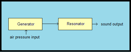
Figure 8. The uncoupled flue pipe physical model described in patent US7442869 by Viscount International
A representation of the flue pipe model described in the Viscount patent is shown in Figure 8. Here there is no coupling or feedback between the generator and resonator, thus the model is an uncoupled one. Because of this the model is clearly not a realistic physical model of an organ pipe. In fact the diagram could just as easily represent simulation by subtractive synthesis (an oscillator followed by a filter) as much as it represents physical modelling. Therefore it is pertinent to enquire how the modelled pipe can emit sound at all in the absence of feedback. The answer is simply because the generator described in the patent is an independent free-running entity which feeds the resonator for as long as a key is held, though this approach does not relate in structural modelling terms to anything found in real organ pipes. Like all other electronic organs, the 'generator' functional block merely models an intermediate generated signal rather than the physical structure within any form of organ pipe, and this is not physical modelling. Uniquely among other synthesis methods, physical modelling as generally understood should model the instrument, not the signals it generates. On the other hand the resonator does employ conventional physical modelling principles. So although the model in Figure 8 is not a complete physical model of a real flue pipe, the simplifications lead to some important practical advantages according to the patent. The patent argues that because the mathematics describing a coupled model is both complicated and nonlinear, deriving sufficiently exact solutions to the equations would require an unrealistic level of computer power. When simulating the organ the high polyphony demand calls for very efficient hardware and software if the system is to run in real time. At the current state of the art this means that with many copies of a coupled pipe model, all of which might be running simultaneously, the patent implies that it would be impossible to solve the equations to the necessary degree of precision. In other words it would not be practical to provide sufficient computing power at a reasonable cost. Therefore it would be unfeasible to calculate values in advance for, say, the oscillator constants in a coupled physical model which correspond exactly to the desired frequency. Hence Viscount's solution, which employs a simplified model with an uncoupled oscillator whose frequency can be set easily and near-instantaneously to an arbitrarily high precision.
Because of this design decision it follows that the model is at a disadvantage in several respects. The attack transient of a flue pipe has been discussed above, and its principal features result from the strong though nonlinear coupling between generator and resonator. For example, the initially anharmonic partials of a transient are pulled into phase-lock to become the exact harmonics of the sound heard during the sustain phase. Without being able to model such coupling only an approximation to the sound of a transient can be achieved, and even this requires empirical adjustment to 'get it right'. Similar remarks apply to release transients. During the sustain phase itself, the intermediate signal applied to the resonator from the generator likewise needs empirical adjusment to approach the desired results. On the other hand an advantage of the system lies in the large number of parameters which are under software control, and some of these are available in the range of voicing options available to the end users of Viscount's products. They illustrate a flexibility which is unfeasible using other simulation techniques. However this brief description of the system confirms the assertion made previously that the overarching problem of physical modelling at the current state of the art lies in its necessary reliance on approximations and simplifications, some of which might be gross. Similar points have been made independently by one of Viscount's competitors (who do not use physical modelling), thus although their views could perhaps be challenged on grounds of impartiality, the following quotation nevertheless seems fair:
" ... note that a model always remains a simplified representation of the reality, which means that the simulation of the chiff and micro-modulations are also very simplified. The big advantage of Physical Modelling is that special effects can be implemented relatively easy [sic] because one can simply modify the computational parameters. However, there is a problem to create the model itself, because there is no connection between the physical parameters and the computational parameters. Designers have to solve this problem by trial and error. When simulating organ pipes it may happen that the designers are not able to find a set of parameters that give a similar sound ... " [16].
This discussion reflects the point made earlier in the article that the issue boils down to simulating particular pipes exactly by sampling their sounds, or simulating a wider range of pipes approximately but more flexibly using physical modelling.
This article has shown how sound is produced by a flue pipe as a result of the closely-coupled interaction between a generator and a resonator. The generator is the air jet issuing from the flue and the resonator is the air enclosed within the body of the pipe. When the pipe is speaking in its sustained tone regime vigorous standing waves are set up in the resonator, and the resulting acoustic field at the mouth impresses a wave-like motion on the air jet as it travels towards the upper lip. The upwards-travelling wave causes the tip of the jet to flip in and out of the pipe across the upper lip, thereby injecting periodic pulses of air into the resonator. A proportion of the energy contained in the pressure and volume flow rate of the injected pulses is transferred to the air column to maintain the standing wave by compensating for its energy losses. The jet moves sinusoidally back and forth across the lip, and although a sine wave contains no harmonics beyond its fundamental frequency, the oscillatory process taken as a whole is nonlinear because the pulses of air injected into the resonator are non-sinusoidal in terms of air pressure and flow. This results in harmonics in the pulse train which are then shaped by the filtering action of the natural resonances of the air column, which form an asymmetrical comb filter. The asymmetry exists because the resonances are anharmonic owing to the variation of the end correction of the pipe with frequency.
This is the basic speaking mechanism of a flue pipe which a physical model must address. However the summary above is simplified, and there also are additional factors which a successful model should incorporate. They include the generation of attack and release transients, and how the sound from the pipe emerges to form a sound wave in the surrounding atmosphere. These latter aspects include the radiating efficiency of the pipe, the non-isotropic acoustic beams arising from its mouth and top, and monopole versus dipole radiation effects specific to stopped and open pipes respectively. All these phenomena are frequency dependent and thus they affect each harmonic in the sound differently. They also depend on the pipe dimensions and its position relative to the listener in three dimensions. Modelling them enables the important directional tone quality of a pipe within an auditorium to be simulated and varied as desired.
The overarching problem of physical modelling lies in its necessary reliance on the approximations which have been identified in this article. Some of the processes outlined above are imperfectly understood, or they involve intractable mathematics which is not well suited to real time synthesis on small computers. Even if this were not the case, all problems in aerodynamics are fundamentally insoluble at a detailed, rigorous level because the underlying Navier-Stokes equations cannot be solved either. The situation does not signify a total impasse by any means, but it implies that physical modelling is a better synthesis technique in some cases than in others. For instance, the simulation of every pipe in a specific organ is probably best realised using sampled sound synthesis, because this gets round the approximation problem simply by recording the actual pipe sounds directly. It is difficult to argue that the sounds of real pipes can be improved by any form of modelling, so when the samples are subsequently replayed by the performer one has a more or less exact reproduction of the sounds of the original instrument. However there are inflexibilities inseparable from any sample set, such as that related to the fixed microphone position at which the samples were recorded. These inflexibilities do not apply nearly as strongly to physical modelling because the range of parameters which can be adjusted in a good model allow spatial effects, for example, to be modified at will. Thus the simulated listening or microphone position can be adjusted within wide limits. On the other hand, the approximate nature of physical modelling means that it cannot approach the sound of a particular pipe at a particular listening position as closely as does sampled sound synthesis. Thus the issue boils down to simulating particular pipes exactly by sampling their sounds, or simulating a wider range of pipes approximately using physical modelling. Both techniques have their place, and ultimately the choice between them must lie with the customer. Therefore it is hoped this article might have illuminated the issues which need to be addressed regarding physical modelling.
1. "How the Flue Pipe Speaks", C E Pykett, 2001 (an article on this website).
2. "The Tonal Structure of Organ Flutes", C E Pykett, 2003 (an article on this website).
3. "The Tonal Structure of Organ Principals", C E Pykett, 2006 (an article on this website).
4. "The Tonal Structure of Organ Strings", C E Pykett, 2012 (an article on this website).
5. "Physical Modelling in Digital Organs", C E Pykett, 2009 (an article on this website).
6. "The Physics of Musical Instruments", N H Fletcher and T D Rossing, corrected 2nd edition, Springer, 1999
7. The speed of the jet issuing from the flue slit is frequently assumed to depend only on blowing pressure in the physical modelling literature, whereas in reality it also depends on flue area. This is no different to the familiar garden hose in which the water speed emerging from the nozzle depends on nozzle size. If it did not, there would be no point buying hose accessories which enable the size to be varied! In both cases the discrepancy is explained by the upstream flow restriction arising at the foot hole of the pipe, which is equivalent to the water flow restriction imposed by the long and narrow garden hose. Thus varying the flue area changes the pressure just below the languid owing to the restrictive action of the foot hole, and it is this sub-languid pressure value which determines jet speed - not the pressure upstream of the foot hole in the chest. This shows why it is so important not to omit the foot hole when modelling an organ pipe, otherwise the entire model can become unrealistic.
8. It is emphasised elsewhere in the main text that reflections which occur transversely across a pipe, especially in the mouth region, imply that the pipe should be treated as a 3-dimensional cavity resonator rather than the 1-dimensional approximation which is usually employed. Unless this is done, the asymmetrical environment of the air jet cannot be modelled, and factors such as the variation of end correction with pipe scale will also continue to elude analysis. The latter plays an important role in defining the frequencies, amplitudes and Q-factors of the anharmonic natural resonances of the pipe. In turn, these exert a strong influence on its timbre or tone colour.
9. "The end corrections, natural frequencies, tone colour and physical modelling of organ pipes", C E Pykett, 2013 (an article on this website).
10. While a pipe is speaking its waveform is exactly periodic (cyclically repeating) or very nearly so. This means the waveform can be decomposed into its constituent harmonics by computing its Fourier series. The frequencies of the harmonics in the Fourier series are always - by definition - exact integer multiples of that of the fundamental, thus no other frequencies can exist. If the fundamental frequency varies slightly, as it might do if the wind pressure fluctuates randomly for some reason, the frequencies of all the harmonics vary in the same way so that they always remain exactly harmonically related. There are no non-harmonically related (anharmonic) frequencies in the sound emitted by an organ pipe other than those constituting any random components it might possess such as wind noise. This is quite different to the significantly anharmonic natural frequencies of the air column, but we do not actually hear these. These facts are laboured here without apology because they seem to create widespread confusion and misunderstanding. For example, one sometimes sees statements such as "this organ builder encouraged the formation of harmonics which are not part of the harmonic series". Such statements are nonsense.
11. The oscillating jet injects pulses of air into the body of the pipe with particular values of pressure and speed (air flow rate). Pressure represents potential energy and speed represents kinetic energy, and it is this energy from the jet which maintains the speech of the pipe by compensating for losses in the resonating air column such as friction between the air molecules and drag at the pipe walls. A physical model must assign values to the relative amounts of potential and kinetic energy transferred, which amounts to computing the phase angle of the oscillation cycle at which the energy transfer takes place, and this represents a significant challenge to achieving a successful model. The problem is similar to designing the escapement of a mechanical pendulum clock, in which the pendulum is the resonator which defines the oscillation frequency but which is also an absorber of energy from the escapement to keep the pendulum moving. The clock designer must decide at which point in the oscillation cycle the escapement transfers its energy to the pendulum, that is, at which point the clock 'ticks'. When the pendulum is at the extremities of its swing its potential energy is at its maximum, and at the base of its swing its kinetic energy is maximised. Achieving the optimum energy injection point from escapement to pendulum (i.e. the optimum phase angle of the oscillation cycle) is critical to the design of a good clock.
In both organ pipes and clocks there is another related issue which concerns the Q-factor of the system (Q defines the sharpness of resonance). For a clock, a high value of Q means it will be a better timekeeper whereas for an organ pipe it means (among other things) the pitch of the pipe will vary less with fluctuations in blowing pressure.
12. "Voicing Electronic Organs", C E Pykett, 2003 (an article on this website).
13. "A Second in the Life of a Violone", C E Pykett, 2005 (an article on this website).
14. "Wet or Dry Sampling for Digital Organs?", C E Pykett, 2010 (an article on this website).
15. "Viscount Organs - some observations on physical modelling patent US7442869", C E Pykett, 2016 (an article on this website).
16. See page 5 entitled "Three Technologies" in 'Organ News no. 23' at www.copemanhart.co.uk/files/Downloads-downloadFile-48.pdf (accessed 16 February 2017).
|